§ Tutorial: solving the Poisson's equation with Medusa

The aim of this tutorial is to introduce basic PDE solving techniques using the Medusa library. The reader will be guided through the stages of solving a PDE, namely domain discretization, choosing the approximation, translating the mathematical formulation of a problem to C++ code, and finally solving the problem. All of this will be done by solving the Poisson's equation i.e. the "Hello, World!" of partial differential equations.

§ Problem

Our considered problem will be taken from the fundamentals of numerical PDE solving, the boundary value problem for the Poisson's equation: $$ \begin{align*} \nabla^2 u &= f && \text{in } \Omega, \\ u &= g && \text{on } \partial \Omega. \end{align*} $$ We will be solving the equation in two dimensions for the sake of simplicity and ease of visualization. While the problem may look simple and timid at first glance, the Poisson's equation finds uses in many physical contexts, be it a standalone problem in potential theory (Newtonian gravity and Electrostatics), heat transfer or just a step in a larger problem such as solving the Navier-Stokes equation or surface reconstruction. It is also found in seemingly unlikely places such as image smoothing.

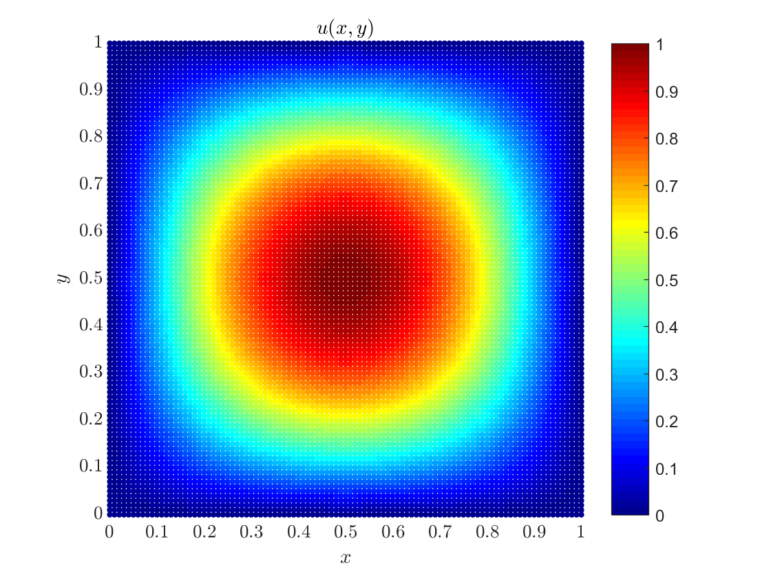
The concrete example we will conside is $$\Omega = [0, 1]\times [0, 1], \quad f(x, y) = -2\pi^2\sin(\pi x)\sin(\pi y), \quad g(x, y) = 0.$$ The solution to this problem is $u(x, y) = \sin(\pi x)\sin(\pi y)$.

§ Method

The generality of approximations in Medusa allows for easy reproduction of many well established strong-form mesh-free methods, such as Diffuse Approximate Method (DAM), Local Radial Basis Function Collocation Methods (LRBFCM), Generalized FDM, Finite Point Method (FPM), Radial Basis Function-generated Finite Differences (RBF-FD), Collocated Discrete Least Squares (CDLS). etc. Many of these can be viewed as a special case of a single method, named simply Meshless Local Strong Form Method (MLSM). Here we will discuss the basic steps of the method to give an intuitive overview in order for us to better understand the solution of the problem at hand, however, further discussion and method details can be found on our wiki.

As opposed to methods like the Finite Element Method (FEM), there is no mesh generation when using meshless methods. Instead, only nodes on the boundary and in the interior are used as discretization points. Each node is assigned a neighbourhood, called its support (the term originates from FEM-like methods, where those nodes actually define a support domain of a trial function) or stencil (the term analogous to FDM). The required differential operators at a given node are approximated as a weighted sum of function values in supporting nodes. For now it will suffice to understand that the method approximates a linear operator $\mathcal{L}$ at a node $p$ as a linear combination of the values of the function at the $n$ closest neighbours: $$ (\mathcal{L}u)(p) \approx \sum_{i=1}^{n} w_i u_i $$ The inner workings of the method are presented here.

The solution procedure can be summarized in four steps.

1. Define, discretize and populate the domain with nodes.
2. Find support for the nodes, define the approximation engine and compute operator shapes.
3. Formulate the problem by filling the problem matrix $M$ and the right hand side with weights $w_i$ and boundary conditions.
4. Solve the resulting system of equations and visualize the solution.

This applies to solving PDEs implicitly, which is customary for the Poisson problem. However steps 1 and 2 don't change considerably for explicit solving. Examples of problems solved explicitly can be found here. We will now discuss the steps 1—4 in detail while writing our first program. One of the best features of Medusa is the simplicity and readability of the code, all while providing high performance.

§ Implementation

If you haven't already, make sure to include the medusa library in your project.

§ Step 1: Define, discretize and populate the domain with nodes

The code for the first step looks like this:

// Create the domain and discretize it.
BoxShape<Vec2d> box(0.0, 1.0);
DomainDiscretization<Vec2d> domain = box.discretizeWithStep(0.01);
domain.findSupport(FindClosest(9));  // Find 9 closest nodes as the support of each node.

Our first course of action is to construct a DomainShape, that represents our domain $\Omega$, in this case the BoxShape is an appropriate choice. We pass Vec2d as the template parameter, because we want to to solve the problem in a two dimensional box (a square) and using doubles for numerical computations. We could solve the problem on a circle if we use CircleShape or pass Vec3d as a parameter to solve it in 3 dimensions.

In this example we will fill the domain uniformly, hence we define a constant step size. In many cases, however, nodal densities are tailored to the problem at hand, to increase accuracy or achieve better convergence, which is also supported by the library. The domain along with the discretization nodes is represented by the DomainDiscretization class. Domain discretization consists of points in the interior and on the boundary. Each point has an associated type, with types of internal points being positive and types of boundary points being negative. Boundary points also have an outer unit normal associated with them.

Finally, a support domain is stored for each node in the domain. The support domain is computed in the last line of the code above and stores the indices of 9 closest neighbouring nodes. To construct stable and reliable approximations the support domains need to be non-degenerate, meaning that the distances between support nodes have to balanced. At the moment we are solving the problem on a very nicely populated domain, however when dealing with more difficult geometries, different fill or regularization engines can be used.

§ Step 2: Define the approximation engine and compute the shape function

In the second step we define the approximation of our linear operator $\mathcal{L}$ and compute it at all nodes. The code looks like this:

// Construct the approximation engine, using monomials and no weight.
int m = 2;  // tensor basis of order 2, {1, x, x^2, y, yx, yx^2, y^2, y^2x, y^2x^2}
WLS<Monomials<Vec2d>, NoWeight<Vec2d>, ScaleToFarthest> wls(Monomials<Vec2d>::tensorBasis(m));

// Compute the shapes and store them (we only need the Laplacian) using our engine.
auto storage = domain.computeShapes<sh::lap>(wls);

// Allocate matrix and right hand side.
Eigen::SparseMatrix<double, Eigen::RowMajor> M(N, N);
M.reserve(storage.supportSizes());
Eigen::VectorXd rhs(N); rhs.setZero();

// Construct implicit operators over our storage.
auto op = storage.implicitOperators(M, rhs);

§ Step 3: Translate the mathematical formulation to C++ code

This step is where the expressive power of Medusa is best seen. We formulate the problem as shown below:

for (int i : domain.interior()) {
    double x = domain.pos(i, 0);
    double y = domain.pos(i, 1);
    // Set the equation in the interior nodes.
    op.lap(i) = -2*PI*PI*std::sin(PI*x)*std::sin(PI*y);
}
for (int i : domain.boundary()) {
    // Enforce the boundary conditions in boundary nodes.
    op.value(i) = 0.0;
}

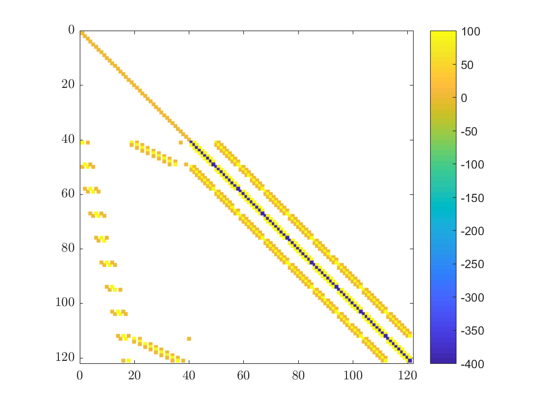
Sparse Matrices

When solving PDEs we often deal with very large matrices in which most of the elements are zero. Such matrices arise when dealing with systems where every variable is coupled only with a few others, in our case an individual node only “interacts” with its support. Our matrix can be seen in the figure below. With the use of specialized iterative algorithms, large sparse systems can be solved efficiently.

§ Step 4: Solve the resulting system of equations and visualize the solution

We use Eigen's implementation of BiCGStab algorithm with ILUT preconditioning to solve the system and the solution is written into a text file for quick processing.

Eigen::BiCGSTAB<decltype(M), Eigen::IncompleteLUT<double>> solver;
solver.compute(M);
ScalarFieldd u = solver.solve(rhs);

// Write the solution into file
std::ofstream out_file("poisson_dirichlet_2D_data.m");
out_file << "positions = " << domain.positions() << ";" << std::endl;
out_file << "solution = " << u << ";" << std::endl;
out_file.close();

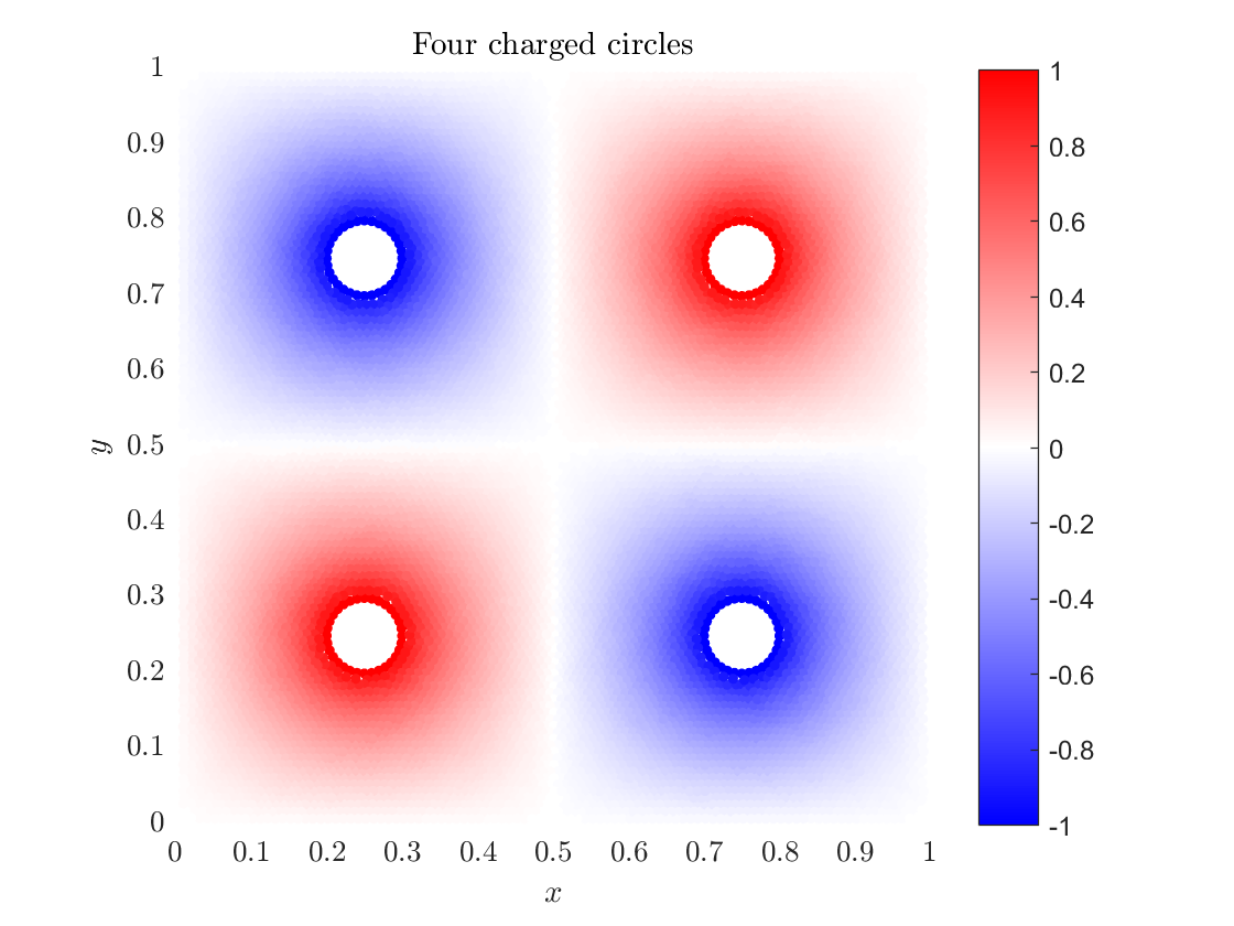
§ Electrostatic quadrupole example

With our knowledge of solving the Poisson's equation we can calculate the Coulomb potential of four charged balls that are positioned on the vertices of a square. Assuming there is no current and the charge distribution is time independent, the electric field $E$ satisfies: $$\nabla\cdot E = \rho/\varepsilon, \quad \nabla \times E = 0,$$ where $\rho$ is the charge density and $\epsilon$ is the permittivity. If we introduce an electrostatics potential $\phi$ such that $$E = -\nabla\phi,$$ we can insert it into the first equation, resulting in Poisson's equation: $\nabla^2 \phi = -\rho/\varepsilon.$ In the absence of unpaired electric charge equation becomes Laplace's equation $$\nabla^2 \phi = 0.$$

Program files for both this and the previous example are available here as quadrupole.cpp and poisson_dirichlet_2D.cpp respectively. Post processing script is written in the poisson_dirichlet_2D.m file.