§ Features

§ Expressiveness and simplicity

Medusa aims to express the mathematical model in C++ code as intuitively, clearly and concisely as possible. Apart from the demo on the home page, three more examples are featured here.

§ Advection-diffusion equation

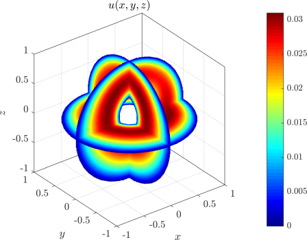
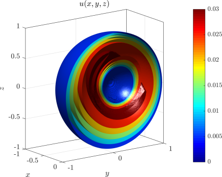
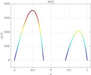
First, let's look at a steady state advection-diffusion equation: $$8 \, (-1, -1, -1) \cdot \nabla u + 2 \, \nabla^2 u = -1$$ on a domain with a hole with Dirichlet boundary conditions $u = 0$. Compare the above equation to the C++ code:

for (int i : domain.interior()) {
    8.0*op.grad(i, {-1, -1, -1}) + 2.0*op.lap(i) = -1.0;
}
for (int i : domain.boundary()) {
    op.value(i) = 0.0;
}

§ Navier-Stokes equations show / hide content

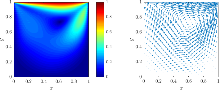
Second, the incompressible Navier-Stokes equations: $$\begin{align*} \frac{\partial \boldsymbol{v}}{\partial t}+ (\boldsymbol{v} \cdot \nabla) \, \boldsymbol{v} &= -\frac{1}{\rho }\nabla p+\nu \nabla^2 \boldsymbol{v}+\boldsymbol{f} \\ \nabla \cdot \boldsymbol{v} &= 0 \end{align*} $$ The classical lid-driven cavity problem was solved. The solution procedure uses explicit Euler time stepping and ACM. It is expressed in Medusa as follows:

for (int step = 0; step <= max_steps; ++step) {
    // Advance velocity
    for (int i : interior)
        v2[i] = v1[i] + dt * (- 1/rho * op.grad(P1, i) + mu/rho * op.lap(v1, i) - op.grad(v1, i) * v1[i]);
    }
    // Pressure correction
    for (auto i : interior) {
        P2[i] = P1[i] - dl * dt * rho * op.div(v2, i) + dl2 * dl * dt * dt * op.lap(P1, i);
    }
    v1.swap(v2);
    P1.swap(P2);
}

The steady state velocity magnitude and vector are are shown in the figure below.

More examples from fluid dynamics can be found here.

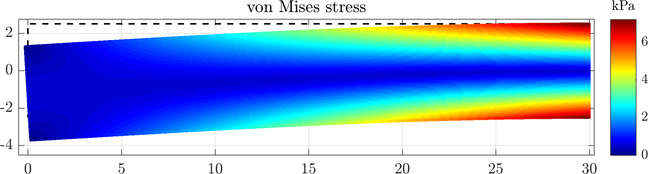
§ Cantilever beam show / hide content

Another example is from linear elasticity, the Navier-Cauchy equation, describing small deformations of materials under load. It reads as $$ (\lambda + \mu) \nabla(\nabla \cdot \boldsymbol{u}) + \mu \nabla^2 \boldsymbol{u} + \boldsymbol{f} = 0 $$ and one of the most famous cases is the cantilever beam problem. The following boundary conditions are applied: $$ \begin{align*} \boldsymbol{u}|_{\text{right}} &= \left(\frac{Py (3D^2(1+\nu) - 4(2+\nu) y^2)}{24 E I}, -\frac{L \nu P y^2}{2 E I}\right), \\ \boldsymbol{\sigma}|_{\text{top}} &= \boldsymbol{\sigma}|_{\text{bottom}} = 0, \\ \boldsymbol{\sigma}|_{\text{left}} &= \left(0, \frac{P}{2 I} \left(D^2/4-y^2\right)\right). \end{align*} $$ The source code in Medusa, taken directly from the library's unit tests suite:

for (int i : domain.interior()) {
    (lam+mu)*op.graddiv(i) + mu*op.lap(i) = 0.0;
}
for (int i : domain.types() == RIGHT) {
    double y = domain.pos(i, 1);
    op.value(i) = {(P*y*(3*D*D*(1+v) - 4*(2+v)*y*y)) / (24.*E*I), -(L*v*P*y*y) / (2.*E*I)};
}
for (int i : domain.types() == LEFT) {
    double y = domain.pos(i, 1);
    op.traction(i, lam, mu, {-1, 0}) = {0, -P*(D*D - 4*y*y) / (8.*I)};
}
for (int i : domain.types() == TOP) {
    op.traction(i, lam, mu, {0, 1}) = 0.0;
}
for (int i : domain.types() == BOTTOM) {
    op.traction(i, lam, mu, {0, -1}) = 0.0;
}

The solution obtained using above code is shown below.

More examples solving the Navier-Cauchy equation can be found here.

§ Simple analyses of various setups

Many common strong-form mesh-free approximations can be seamlessly changed: discrete least squares, collocation, Radial Basis Function-generated finite differences, monomial augmentation, etc.

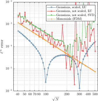
Approximations can be easily defined and changed. You can control types of RBFs, dimension of the space, monomial augmentation, shape parameters, scaling, system solvers...

RBFFD<Polyharmonic<double>, Vec2d, ScaleToClosest> approx(3, Monomials<Vec2d>(2));
WLS<MQs<Vec3d>, GaussianWeight<Vec3d>, NoScale, Eigen::PartialPivLU<Eigen::MatrixXd>> wls({9, 1.5}, 0.8);

§ Node generation

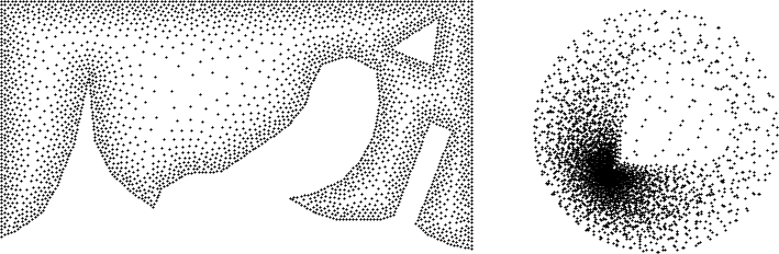
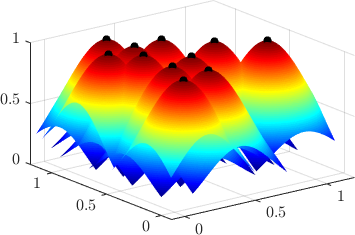
We support variable density node generation in any dimension with various node generation algorithms and spatial search structures as well as post processing iterative improvement techniques. However, you can also generate regularly spaced nodes on a unit square, for example.

§ Dimension independence

Our aim is to have the code as dimension agnostic as possible. This is why most of our code, such as the node generation algorithms, approximation methods and solution procedures work in arbitrary dimensions.

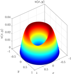
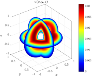
The solution of the advection-diffusion equation from the top of the page is shown here, using the same code as above in all dimensions. The source code is available here along with other Medusa examples. If care is taken, the dimension of the problem can be a runtime parameter.

§ Utilities

The library is divided into modules, whose precise contents are listed in the modules page of the API reference. Main parts are showcased here.

§ Domains

The library directly supports circular and rectangular domains in all three dimensions. Additionally, We support 2D polygons and arbitrary union/difference/affine transformation of all these. We also support parametrically given domains (including NURBS). Any such domain can be discretized with respect to any nodal spacing function or a discretization obtained elsewhere can be loaded from a file.

§ Approximations

Many common strong-form mesh-free approximations can be seamlessly changed: discrete least squares, collocation, Radial Basis Functions generated finite differences, monomial augmentation … Every part of the approximation procedure is modular and fully customizable.

§ Operators

Discretized differential operators in Medusa allow for elegant code that very closely resembles the mathematical formulation. Nonetheless, the user has access to coordinate derivatives to assemble any operator and to all fields and linear systems involved.

§ Miscellaneous

§ Extensibility

§ Speed