Difference between revisions of "Weighted Least Squares (WLS)"
| Line 8: | Line 8: | ||
\[\hat u({\bf{p}}) = \sum\limits_i^m {{\alpha _i}{b_i}({\bf{p}})} = {{\bf{b}}^{\rm{T}}}{\bf{\alpha }}\] | \[\hat u({\bf{p}}) = \sum\limits_i^m {{\alpha _i}{b_i}({\bf{p}})} = {{\bf{b}}^{\rm{T}}}{\bf{\alpha }}\] | ||
where $\hat u,\,{B_i}\,and\,{\alpha _i}$ stand for approx. function, coefficients and basis function, respectively. We minimize the sum of residuum squares, i.e., the sum of squares of difference between the approx. function and target function, in addition we can also add weight function that controls the significance of nodes, i.e., | where $\hat u,\,{B_i}\,and\,{\alpha _i}$ stand for approx. function, coefficients and basis function, respectively. We minimize the sum of residuum squares, i.e., the sum of squares of difference between the approx. function and target function, in addition we can also add weight function that controls the significance of nodes, i.e., | ||
| − | [{ | + | \[{r^2} = \sum\limits_j^n {W\left( {{{\bf{p}}_j}} \right){{\left( {u({{\bf{p}}_j}) - \hat u({{\bf{p}}_j})} \right)}^2}} = {\left( {{\bf{B\alpha }} - {\bf{u}}} \right)^{\rm{T}}}{\bf{W}}\left( {{\bf{B\alpha }} - {\bf{u}}} \right)\] |
| − | |||
| − | |||
| − | |||
| − | |||
| − | |||
| − | |||
| − | |||
| − | |||
| − | |||
| − | |||
| − | |||
| − | |||
| − | |||
| − | |||
| − | |||
| − | |||
| − | |||
| − | |||
| − | |||
| − | |||
| − | |||
| − | |||
| − | |||
| − | |||
| − | |||
| − | |||
| − | |||
| − | |||
| − | |||
| − | |||
| − | |||
| − | |||
| − | |||
| − | |||
| − | |||
| − | |||
| − | |||
| − | |||
| − | |||
| − | |||
| − | |||
| − | |||
| − | |||
| − | |||
| − | |||
| − | |||
| − | |||
| − | |||
| − | |||
| − | |||
| − | |||
| − | |||
| − | |||
| − | |||
| − | |||
| − | |||
| − | |||
| − | |||
| − | |||
| − | |||
| − | |||
| − | |||
| − | |||
| − | |||
| − | |||
| − | |||
| − | |||
| − | |||
| − | |||
| − | |||
| − | |||
Revision as of 18:23, 20 October 2016
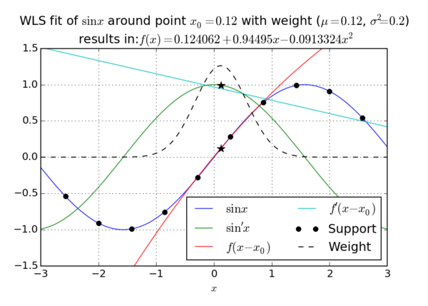
One of the most important building blocks of the meshless methods is the Moving Least Squares approximation, which is implemented in the EngineMLS class.
In general, approximation function can be written as \[\hat u({\bf{p}}) = \sum\limits_i^m {{\alpha _i}{b_i}({\bf{p}})} = {{\bf{b}}^{\rm{T}}}{\bf{\alpha }}\] where $\hat u,\,{B_i}\,and\,{\alpha _i}$ stand for approx. function, coefficients and basis function, respectively. We minimize the sum of residuum squares, i.e., the sum of squares of difference between the approx. function and target function, in addition we can also add weight function that controls the significance of nodes, i.e., \[{r^2} = \sum\limits_j^n {W\left( {{{\bf{p}}_j}} \right){{\left( {u({{\bf{p}}_j}) - \hat u({{\bf{p}}_j})} \right)}^2}} = {\left( {{\bf{B\alpha }} - {\bf{u}}} \right)^{\rm{T}}}{\bf{W}}\left( {{\bf{B\alpha }} - {\bf{u}}} \right)\]
