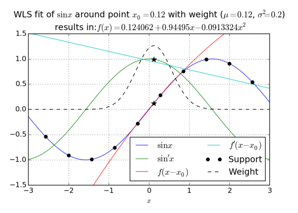
Weighted Least Squares (WLS)

One of the most important building blocks of the meshless methods is the Weighted/Moving Least Squares (WLS/MLS) approximation , which is implemented in the WLS class. It is also often called GFDM (generalized finite differences method).

Notation cheat sheet

\begin{align*} m \in \N & \dots \text{number of basis functions} \\ n \geq m \in \N & \dots \text{number of points in support domain} \\ k \in \mathbb{N} & \dots \text{dimensionality of vector space} \\ \vec s_j \in \R^k & \dots \text{point in support domain } \quad j=1,\dots,n \\ u_j \in \R & \dots \text{value of function to approximate in }\vec{s}_j \quad j=1,\dots,n \\ \vec p \in \R^k & \dots \text{center point of approximation} \\ b_i\colon \R^k \to \R & \dots \text{basis functions } \quad i=1,\dots,m \\ B_{j, i} \in \R & \dots \text{value of basis functions in support points } b_i(\vec{s}_j) \quad j=1,\dots,n, \quad i=1,\dots,m\\ \omega \colon \R^k \to \R & \dots \text{weight function} \\ w_j \in \R & \dots \text{weights } \omega(\vec{s}_j-\vec{p}) \quad j=1,\dots,n \\ \alpha_i \in \R & \dots \text{expansion coefficients around point } \vec{p} \quad i=1,\dots,m \\ \hat u\colon \R^k \to \R & \dots \text{approximation function (best fit)} \\ \chi_j \in \R & \dots \text{shape coefficient for point }\vec{p} \quad j=1,\dots,n \\ \end{align*}

We will also use \(\b{s}, \b{u}, \b{b}, \b{\alpha}, \b{\chi} \) to denote a column of corresponding values, $W$ as a $n\times n$ diagonal matrix filled with $w_j$ on the diagonal and $B$ as a $n\times m$ matrix filled with $B_{j, i} = b_i(\vec s_j)$.

Definition of local approximation

Figure 1: Example of 1D WLS approximation

Our wish is to approximate an unknown function $u\colon \R^k \to \R$ while knowing $n$ values $u(\vec{s}_j) := u_j$. The vector of known values will be denoted by $\b{u}$ and the vector of coordinates where those values were achieved by $\b{s}$. Note that $\b{s}$ is not a vector in the usual sense since its components $\vec{s}_j$ are elements of $\R^k$, but we will call it vector anyway. The values of $\b{s}$ are called nodes or support nodes or support. The known values $\b{u}$ are also called support values.

In general, an approximation function around point $\vec{p}\in\R^k$ can be written as \[\hat{u} (\vec{x}) = \sum_{i=1}^m \alpha_i b_i(\vec{x}) = \b{b}(\vec{x})^\T \b{\alpha} \] where $\b{b} = (b_i)_{i=1}^m$ is a set of basis functions, $b_i\colon \R^k \to\R$, and $\b{\alpha} = (\alpha_i)_{i=1}^m$ are the unknown coefficients.

In MLS the goal is to minimize the error of approximation in given values, $\b{e} = \hat u(\b{s}) - \b{u}$ between the approximation function and target function in the known points $\b{x}$. The error can also be written as $B\b{\alpha} - \b{u}$, where $B$ is rectangular matrix of dimensions $n \times m$ with rows containing basis function evaluated in points $\vec{s}_j$. \[ B = \begin{bmatrix} b_1(\vec{s}_1) & \ldots & b_m(\vec{s}_1) \\ \vdots & \ddots & \vdots \\ b_1(\vec{s}_n) & \ldots & b_m(\vec{s}_n) \end{bmatrix} = [b_i(\vec{s}_j)]_{j=1,i=1}^{n,m} = [\b{b}(\vec{s}_j)^\T]_{j=1}^n. \]

We can choose to minimize any norm of the error vector $e$ and usually choose to minimize the $2$-norm or square norm \[ \|\b{e}\| = \|\b{e}\|_2 = \sqrt{\sum_{j=1}^n e_j^2}. \] Commonly, we also choose to minimize a weighted norm instead \[ \|\b{e}\|_{2,w} = \|\b{e}\|_w = \sqrt{\sum_{j=1}^n (w_j e_j)^2}. \] The weights $w_i$ are assumed to be non negative and are assembled in a vector $\b{w}$ or a matrix $W = \operatorname{diag}(\b{w})$ and usually obtained from a weight function. A weight function is a function $\omega\colon \R^k \to[0,\infty)$. We calculate $w_j$ as $w_i := \omega(\vec{p}-\vec{s}_j)$, so good choices for $\omega$ are function which have higher values close to $0$ (making closer nodes more important), like the normal distribution. If we choose $\omega \equiv 1$, we get the unweighted version.

A choice of minimizing the square norm gave this method its name - Least Squares approximation. If we use the weighted version, we get the Weighted Least Squares or WLS. In the most general case we wish to minimize \[ \|\b{e}\|_{2,w}^2 = \b{e}^\T W^2 \b{e} = (B\b{\alpha} - \b{u})^\T W^2(B\b{\alpha} - \b{u}) = \sum_j^n w_j^2 (\hat{u}(\vec{s}_j) - u_j)^2 \]

The problem of finding the coefficients $\b{\alpha}$ that minimize the error $\b{e}$ numerically is described in Solving overdetermined systems.

Here, we simply write the solution $\b \alpha = (WB)^+ Wu = (B^\T W^2 B)^{-1} B^\T W^2 u$.

In our WLS engine we use SVD with regularization by default.

Weighted Least Squares

Weighted least squares approximation is the simplest version of the procedure described above. Given support $\b{s}$, values $\b{u}$ and an anchor point $\vec{p}$, we calculate the coefficients $\b{\alpha}$ using one of the above methods. Then, to approximate a function in the neighbourhood of $\vec p$ we use the formula \[ \hat{u}(\vec x) = \b{b}(\vec x)^\T \b{\alpha} = \sum_{i=1}^m \alpha_i b_i(\vec x). \]

To approximate the derivative $\frac{\partial u}{\partial x_i}$, or any linear partial differential operator $\mathcal L$ on $u$, we simply take the same linear combination of transformed basis functions $\mathcal L b_i$. We have considered coefficients $\alpha_i$ to be constant and applied the linearity. \[ \widehat{\mathcal L u}(\vec x) = \sum_{i=1}^m \alpha_i (\mathcal L b_i)(\vec x) = (\mathcal L \b b(\vec x))^\T \b \alpha. \]

Moving Least Squares

Figure 2: Comparison of WLS and MLS approximation

When using WLS the approximation gets worse as we move away from the central point $\vec{p}$. This is partially due to not being in the center of the support any more and partially due to weight being distributed in such a way to assign more importance to nodes closer to $\vec{p}$.

We can battle this problem in two ways: when we wish to approximate in a new point that is sufficiently far away from $\vec{p}$ we can compute new support, recompute the new coefficients $\b{\alpha}$ and approximate again. This is very costly and we would like to avoid that. A partial fix is to keep support the same, but only recompute the weight vector $\b{w}$, that will now assign weight values to nodes close to the new point. We still need to recompute the coefficients $\b{\alpha}$, however we avoid the cost of setting up new support and function values and recomputing $B$. This approach is called Moving Least Squares due to recomputing the weighted least squares problem whenever we move the point of approximation.

Note that if our weight is constant or if $n = m$, when approximation reduces to interpolation, the weights do not play any role and this method is redundant. In fact, its benefits arise when supports are rather large.

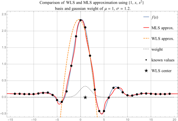
See Figure 2 for comparison between MLS and WLS approximations. MLS approximation remains close to the actual function while still inside the support domain, while WLS approximation becomes bad when we come out of the reach of the weight function.