Difference between revisions of "Weighted Least Squares (WLS)"
(→Basics) |
(→Basics) |
||
| Line 13: | Line 13: | ||
* Normal equation (fastest – less accurate) – using Cholesky decomposition | * Normal equation (fastest – less accurate) – using Cholesky decomposition | ||
| + | * QR decomposition of $\bf{B}$ ($rank(\bf{B})=m$ – number of basis functions) | ||
| + | * SVD decomposition of $\bf{B}$ (more expensive – more reliable, no rank demand) | ||
| + | |||
| + | In MM we use SVD. | ||
| + | |||
| + | == Normal equations | ||
We seek the minimum of | We seek the minimum of | ||
\[{\bf{r}} = {\bf{u}} - {\bf{B\alpha }}\] | \[{\bf{r}} = {\bf{u}} - {\bf{B\alpha }}\] | ||
| Line 20: | Line 26: | ||
resulting in | resulting in | ||
\[{\bf{B}}{{\bf{B}}^{\rm{T}}}{\bf{\alpha }} = {{\bf{B}}^{\rm{T}}}{\bf{u}}\] | \[{\bf{B}}{{\bf{B}}^{\rm{T}}}{\bf{\alpha }} = {{\bf{B}}^{\rm{T}}}{\bf{u}}\] | ||
| − | The coefficient matrix | + | The coefficient matrix $\bf{B}^T\\bf{B}$ is symmetric and positive definite. However, solving above problem directly is |
| − | poorly behaved with respect to round-off effects since the condition number | + | poorly behaved with respect to round-off effects since the condition number of $\bf{B}^T\\bf{B}$is the square |
| − | + | of that of B. Or in case of weighted LS | |
| − | |||
| − | |||
| − | |||
| − | |||
| − | |||
== Shape functions == | == Shape functions == | ||
Revision as of 18:39, 20 October 2016
One of the most important building blocks of the meshless methods is the Moving Least Squares approximation, which is implemented in the EngineMLS class.
Basics
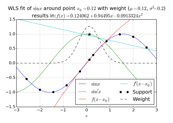
In general, approximation function can be written as \[\hat u({\bf{p}}) = \sum\limits_i^m {{\alpha _i}{b_i}({\bf{p}})} = {{\bf{b}}^{\rm{T}}}{\bf{\alpha }}\] where $\hat u,\,{B_i}\,and\,{\alpha _i}$ stand for approx. function, coefficients and basis function, respectively. We minimize the sum of residuum squares, i.e., the sum of squares of difference between the approx. function and target function, in addition we can also add weight function that controls the significance of nodes, i.e., \[{r^2} = \sum\limits_j^n {W\left( {{{\bf{p}}_j}} \right){{\left( {u({{\bf{p}}_j}) - \hat u({{\bf{p}}_j})} \right)}^2}} = {\left( {{\bf{B\alpha }} - {\bf{u}}} \right)^{\rm{T}}}{\bf{W}}\left( {{\bf{B\alpha }} - {\bf{u}}} \right)\] Where $\bf{B}$ is non-square matrix of dimension $m \times n$ and $\bf{W}$ diagonal matrix of weights. The least squares problem can be solved with three approaches
- Normal equation (fastest – less accurate) – using Cholesky decomposition
- QR decomposition of $\bf{B}$ ($rank(\bf{B})=m$ – number of basis functions)
- SVD decomposition of $\bf{B}$ (more expensive – more reliable, no rank demand)
In MM we use SVD.
== Normal equations We seek the minimum of \[{\bf{r}} = {\bf{u}} - {\bf{B\alpha }}\] \[{r^2} = {\left( {{\bf{u}} - {\bf{B\alpha }}} \right)^{\rm{T}}}\left( {{\bf{u}} - {\bf{B\alpha }}} \right)\] By seeking the zero gradient in terms of coefficient \[\frac{\partial }{{\partial {\alpha _i}}}\left( {{{\left( {{\bf{u}} - {\bf{B\alpha }}} \right)}^{\rm{T}}}\left( {{\bf{u}} - {\bf{B\alpha }}} \right)} \right) = 0\] resulting in \[{\bf{B}}{{\bf{B}}^{\rm{T}}}{\bf{\alpha }} = {{\bf{B}}^{\rm{T}}}{\bf{u}}\] The coefficient matrix $\bf{B}^T\\bf{B}$ is symmetric and positive definite. However, solving above problem directly is poorly behaved with respect to round-off effects since the condition number of $\bf{B}^T\\bf{B}$is the square of that of B. Or in case of weighted LS
