Difference between revisions of "Poisson's equation"
E6WikiAdmin (talk | contribs) |
|||
| (54 intermediate revisions by 4 users not shown) | |||
| Line 1: | Line 1: | ||
| − | + | {{Box-round|title= Related papers | | |
| + | [https://e6.ijs.si/ParallelAndDistributedSystems/publications/52715011.pdf M. Jančič, J. Slak, G. Kosec; Monomial augmentation guidelines for RBF-FD from accuracy versus computational time perspective, Journal of scientific computing, vol. 87, 2021 [DOI: 10.1007/s10915-020-01401-y]] | ||
| + | [https://e6.ijs.si/ParallelAndDistributedSystems/publications/69777155.pdf J. Slak, G. Kosec; Medusa : A C++ library for solving PDEs using strong form mesh-free methods, ACM transactions on mathematical software, vol. 47, 2021 [DOI: 10.1145/3450966]] | ||
| + | }} | ||
| + | |||
| + | __TOC__ | ||
| + | |||
| + | Go back to [[Medusa#Examples|Examples]]. | ||
| + | |||
| + | == Dirichlet boundary conditions == | ||
| + | It is fitting that examples start with a simple case, and we will gradually make our way towards more complicated cases with different domain shapes, boundary conditions and approximation types. | ||
| + | Consider the solution of the 2D Poisson equation on a unit square with Dirichlet boundary conditions: | ||
<math> | <math> | ||
| − | + | \begin{align*} | |
| − | \Delta u = f | + | \Delta u &= f &&\text{in } \Omega, \\ |
| − | + | u &= 0 &&\text{on } \partial \Omega, | |
| − | \end{ | + | \end{align*} |
</math> | </math> | ||
| − | + | where $u(x,y)$ is the solution to the problem, $\Omega = [0, 1] \times [0, 1]$ and in the case we will consider $f(x,y) = -2\pi^2\sin(\pi x)\sin(\pi y)$, as it makes for | |
| − | + | a simple solution $u(x,y) = \sin(\pi x)\sin(\pi y)$. | |
| − | First | + | First, we construct our domain and discretize it, then find support (neighborhood) for each node. |
<syntaxhighlight lang="c++" line> | <syntaxhighlight lang="c++" line> | ||
| Line 22: | Line 33: | ||
</syntaxhighlight> | </syntaxhighlight> | ||
| − | We constructed a box shape, discretized it with a constant step dx (both inside and the boundary) and choose the closest 9 nodes of each node as its support. The next | + | We constructed a box shape, discretized it with a constant step dx (both inside and the boundary) and choose the closest 9 nodes of each node as its support. The next step is to construct our approximation engine. |
| + | Simply put, approximation engines are classes responsible for [[Computation of shape functions|computing shape functions]] for given operator and points. While many different setups are supported in Medusa we will start off simple, | ||
| + | with an approximation that reproduces standard Finite Difference method. | ||
<syntaxhighlight lang="c++" line> | <syntaxhighlight lang="c++" line> | ||
int m = 2 | int m = 2 | ||
| − | WLS<Monomials<Vec2d>, NoWeight<Vec2d>, | + | WLS<Monomials<Vec2d>, NoWeight<Vec2d>, ScaleToFarthest> wls(Monomials<Vec2d>::tensorBasis(m)); |
| − | |||
</syntaxhighlight> | </syntaxhighlight> | ||
| − | We constructed a [[ | + | We constructed a [[Weighted Least Squares (WLS) | WLS]] engine using monomial tensor basis of order 2. Finally, we write the equations for our problem by directly translating |
| + | the mathematical formulation above into code. | ||
<syntaxhighlight lang="c++" line> | <syntaxhighlight lang="c++" line> | ||
for (int i : domain.interior()) { | for (int i : domain.interior()) { | ||
| − | double x = domain.pos(i,0); | + | double x = domain.pos(i, 0); |
| − | double y = domain.pos(i,1); | + | double y = domain.pos(i, 1); |
| − | op.lap(i) = -2* | + | op.lap(i) = -2*PI*PI*std::sin(PI*x)*std::sin(PI*y); |
} | } | ||
for (int i : domain.boundary()) { | for (int i : domain.boundary()) { | ||
| Line 43: | Line 56: | ||
</syntaxhighlight> | </syntaxhighlight> | ||
| − | Here is the plot of the solution for <math>u(x,y)</math> | + | Here is the plot of the solution $u(x, y)$. |
| + | |||
| + | [[File:dirichlet.png|800px]] | ||
| + | |||
| + | The whole example can be found as [https://gitlab.com/e62Lab/medusa poisson_dirichlet_2D.cpp] along with the plot script that can be run by Matlab or Octave [https://gitlab.com/e62Lab/medusa poisson_dirichlet_2D.m]. | ||
| + | Same goes for similar cases solved in 1D and 3D and their respective plot scripts. | ||
| + | |||
| + | == Mixed boundary conditions == | ||
| + | |||
| + | We can obtain the solution to the above problem by solving it on just a quarter of the original domain and using mixed boundary conditions. By using Dirichlet boundary conditions on the bottom and the left side of the square domain, and Neumann boundary conditions on the right and upper side of the domain we are effectively solving the same problem but on a quarter of the domain. Our problem is now: | ||
| + | |||
| + | <math> | ||
| + | \begin{align*} | ||
| + | \Delta u &= f &&\text{in } \Omega, \\ | ||
| + | u &= 0 &&\text{on } \partial \Omega_1 \cup \partial \Omega_3,\\ | ||
| + | \frac{du}{d \b{\hat{n}}} &= 0 &&\text{on } \partial \Omega_2 \cup \partial \Omega_4 | ||
| + | \end{align*} | ||
| + | </math> | ||
| + | |||
| + | Where $\partial \Omega_1$, $\partial \Omega_2$, $\partial \Omega_3$ and $\partial \Omega_4$ are left, right, bottom and top boundary respectively. The domain is $\Omega = [0, 0.5] \times [0, 0.5]$, and $\frac{du}{d \b{\hat{n}}}$ is the normal derivative (on the boundary). | ||
| + | |||
| + | When constructing approximation engines, there are a lot of different options, you can choose between different basis functions, weights, scale functions and each setup comes with its advantages and disadvantages. Some might work for certain problems and some might not. When writing the examples we tried to present the reader with as many different options as possible. | ||
| + | |||
| + | Let us solve the problem using Gaussian RBF (Radial Basis Functions) instead of Monomials: | ||
| + | |||
| + | <syntaxhighlight lang="c++" line> | ||
| + | // shape = 30 | ||
| + | // m = 9 | ||
| + | WLS<Gaussians<Vec2d>, NoWeight<Vec2d>, ScaleToFarthest, | ||
| + | Eigen::LLT<Eigen::MatrixXd>> wls({9, 30}); | ||
| + | </syntaxhighlight> | ||
| + | |||
| + | While the case is the same for the nodes inside the domain, we need to change the boundary conditions: | ||
| + | |||
| + | <syntaxhighlight lang="c++" line> | ||
| + | int BOTTOM = -3; | ||
| + | int TOP = -4; | ||
| + | int LEFT = -1; | ||
| + | int RIGHT = -2; | ||
| + | |||
| + | for (int i : (domain.types() == LEFT) + (domain.types() == BOTTOM)) { | ||
| + | op.value(i) = 0.0; // Dirichlet boundary conditions on the left and bottom edge of the box | ||
| + | } | ||
| + | for (int i : (domain.types() == TOP) + (domain.types() == RIGHT)) { | ||
| + | // Neumann boundary conditions on upper and right edge of the box | ||
| + | op.neumann(i, domain.normal(i)) = 0.0; | ||
| + | } | ||
| + | </syntaxhighlight> | ||
| + | |||
| + | When solving a PDE implicitly a system of equations needs to be solved to obtain the solution. For this, we use [http://eigen.tuxfamily.org/index.php?title=Main_Page Eigen]. | ||
| + | |||
| + | <syntaxhighlight lang="c++" line> | ||
| + | Eigen::BiCGSTAB<decltype(M), Eigen::IncompleteLUT<double>> solver; | ||
| + | solver.compute(M); | ||
| + | ScalarFieldd u = solver.solve(rhs); | ||
| + | </syntaxhighlight> | ||
| + | |||
| + | Matrix M and rhs are the sparse matrix and vector in which we wrote (with the help of Medusa) the system of equations that when solved gives us an approximate solution of our problem. We solve the system using an Eigen linear equation solver, in this case, the BiCGStab algorithm with ILUT preconditioning. The solution is plotted below: | ||
| + | |||
| + | [[File:mixed.png|800px]] | ||
| + | |||
| + | The whole example can be found as [https://gitlab.com/e62Lab/medusa poisson_mixed_2D.cpp] along with the plot script that can be run by Matlab or Octave [https://gitlab.com/e62Lab/medusa poisson_mixed_2D.m]. Similar examples such as mixed boundary conditions on a circular domain, mixed boundary conditions on an irregular domain and a solution to a similar problem using monomial augmentation of radial basis functions can be found [https://gitlab.com/e62Lab/medusa here]. | ||
| + | |||
| + | == Full Neumann boundary conditions == | ||
| + | When solving the Navier-Stokes equation with Explicit Pressure correction, a Poisson's equation with full Neumann boundary conditions needs to be solved. In order for this type of problem to be solved, it needs to satisfy the compatibility condition. Inside the domain we still have: | ||
| + | |||
| + | $$ | ||
| + | \Delta u = f | ||
| + | $$ | ||
| + | |||
| + | The Poisson equation has a solution for the requisite function $u(x,y)$, when the integral of the source function $f(x,y)$ over our domain needs to be equal to the net flow rate, that is expressed by the boundary integral of the normal derivative of $u(x,y)$. In mathematical formulation, for our 2D case: | ||
| + | |||
| + | $$ | ||
| + | \int_{\Omega} f(x,y) dxdy = \int_{\partial \Omega} \frac{du}{d \b{\hat{n}}} dl | ||
| + | $$ | ||
| + | |||
| + | Where again $\Omega$ is our domain, $\partial \Omega$ is the boundary of our domain, $dl$ is the differential arc length along the boundary. When the compatibility condition is met, the Poisson equation has a solution that can be determined up to an arbitrary constant. To obtain only one solution another constraint needs to be implemented. One option is to select a node and set it to a constant, e.g. p(0, 0) = 0, however much more stable approach is to enforce solution with an additional condition, also referred to as a regularization: | ||
| + | |||
| + | $$ | ||
| + | \int_{\Omega }^{{}}{u(x,y)d}\Omega = 0 | ||
| + | $$ | ||
| + | |||
| + | On our unit square domain, $\Omega = [0, 1] \times [0, 1]$ an example case that satisfies the compatibility condition would be: | ||
| + | |||
| + | <syntaxhighlight lang="c++" line> | ||
| + | for (int i : domain.interior()) { | ||
| + | op.lap(i) = 2; | ||
| + | } | ||
| + | |||
| + | int BOTTOM = -3; | ||
| + | int TOP = -4; | ||
| + | int LEFT = -1; | ||
| + | int RIGHT = -2; | ||
| + | |||
| + | for (int i : (domain.types() == LEFT)) { | ||
| + | op.der1(i, 0) = 0.0; | ||
| + | } | ||
| + | for (int i : (domain.types() == RIGHT)) { | ||
| + | op.der1(i, 0) = 1.0; | ||
| + | } | ||
| + | for (int i : (domain.types() == BOTTOM)) { | ||
| + | op.der1(i, 1) = 0.0; | ||
| + | } | ||
| + | for (int i : (domain.types() == TOP)) { | ||
| + | op.der1(i, 1) = 1.0; | ||
| + | } | ||
| + | </syntaxhighlight> | ||
| + | |||
| + | Which is simply, $\Delta u = 2$ inside $\Omega$ while $\frac{du}{d \b{\hat{n}}} = 1$ on top and right boundary and $\frac{du}{d \b{\hat{n}}} = 0$ on the other two. With a little mental math we see that the compatibility condition is met, $2 * 1 = 0 + 1 + 0 + 1$. With that out of the way let us see how we implement regularization: | ||
| + | |||
| + | Well the idea add another line and column to matrix M holding the shape function s, and enforce the condition. We do this by adding a Lagrange multiplier $\alpha$: | ||
| + | |||
| + | $$ | ||
| + | \left[ \begin{matrix} | ||
| + | {{M}_{11}} & .. & {{M}_{1n}} & 1 \\ | ||
| + | .. & .. & .. & 1 \\ | ||
| + | {{M}_{n1}} & ... & {{M}_{nn}} & 1 \\ | ||
| + | 1 & 1 & 1 & 0 \\ | ||
| + | \end{matrix} \right]\left[ \begin{matrix} | ||
| + | {{u}_{1}} \\ | ||
| + | ... \\ | ||
| + | {{u}_{n}} \\ | ||
| + | \alpha \\ | ||
| + | \end{matrix} \right]=\left[ \begin{matrix} | ||
| + | rhs_1 \\ | ||
| + | ... \\ | ||
| + | rhs_n \\ | ||
| + | 0 \\ | ||
| + | \end{matrix} \right] | ||
| + | $$ | ||
| + | |||
| + | When the problem is well-posed $\alpha$ should be equal to zero, or at least very close. Let us fill our matrix M: | ||
| + | |||
| + | <syntaxhighlight lang="c++" line> | ||
| + | // regularization | ||
| + | // set the last row and column of the matrix | ||
| + | for (int i = 0; i < N; ++i) { | ||
| + | M.coeffRef(N, i) = 1; | ||
| + | M.coeffRef(i, N) = 1; | ||
| + | } | ||
| + | // set the sum of all values | ||
| + | rhs[N] = 0.0; | ||
| + | </syntaxhighlight> | ||
| + | |||
| + | If we take a look at the matrix we will see the extra row and column that enforce our constraint. They should be the last column and the last row of the matrix: | ||
| + | |||
| + | [[File:sparse_neumann_problem.png|800px]] | ||
| + | |||
| + | With this done we can solve the problem, just as we did in the examples above. | ||
| + | |||
| + | [[File:poisson_neumann_2D.png|800px]] | ||
| + | |||
| + | For $dx = 0.05$ we get $\alpha = -1.03846 \cdot 10^{-13}$, which is expected from a valid solution. | ||
| + | |||
| + | The whole example can be found as [https://gitlab.com/e62Lab/medusa poisson_neumann_2D.cpp] along with the plot script that can be run by Matlab or Octave [https://gitlab.com/e62Lab/medusa poisson_neumann_2D.m]. | ||
| + | |||
| + | == 3D model case == | ||
| + | |||
| + | A 3D domain <code>triceratops.h5</code> was created from the Mathematica's triceratops model. The point coordinates can be imported to medusa and used as a domain. In the example given in <code>triceratops.cpp</code> | ||
| + | the equation $-\nabla^u = 1$ with $u=0$ on the boundary is solved. | ||
| + | |||
| + | The plot of the solution obtained using <code>triceratops.m</code> is shown below: | ||
| + | |||
| + | [[File:triceratops_example.png|800px]] | ||
| + | |||
| + | == Convergence rate - including high order solution == | ||
| + | Assume a $d$-dimensional Poisson problem with mixed boundary conditions. | ||
| + | |||
| + | <math> | ||
| + | \begin{align*} | ||
| + | \nabla ^2 u(\boldsymbol x) &= -d \pi ^2 \prod_{i=1} ^d \sin(\pi x_i) \qquad &&\text{in } \Omega, \\ | ||
| + | u(\boldsymbol x) &= \prod _{i = 1} ^d \sin(\pi x_i) \qquad && \text{on } \Gamma_d,\\ | ||
| + | \frac{\partial u}{\partial \boldsymbol n}(\boldsymbol x) &= \pi \sum_{i=1}^d n_i \cos(\pi x_i) \prod_{j\neq i} \sin(\pi x_j) | ||
| + | \qquad && \text{on } \Gamma_n, | ||
| + | \end{align*} | ||
| + | </math> | ||
| + | |||
| + | where $n_i$ are components of the unit normal vector $\boldsymbol n$, $\Omega$ is a $d$-dimensional ball with origin at $\boldsymbol x = \boldsymbol{1} \boldsymbol{/} \boldsymbol{2}$ and radius $r = 1/2$, and $\Gamma_d$, $\Gamma_n$ are left and right halves of the boundary, respectively: | ||
| + | |||
| + | <math> | ||
| + | \begin{align*} | ||
| + | \Omega &= \left\{ \boldsymbol x, \ \left\|\boldsymbol x - \boldsymbol{\frac 1 2}\right\| < \frac 1 2 \right\}, \\ | ||
| + | \Gamma_d &= \left \{ \boldsymbol x \in \partial \Omega,\boldsymbol x_1 < \frac 1 2 \right \}, \\ | ||
| + | \Gamma_n &= \left \{ \boldsymbol x \in \partial \Omega,\boldsymbol x_1 \geq \frac 1 2 \right \}. | ||
| + | \end{align*} | ||
| + | </math> | ||
| + | |||
| + | Solution of the above case is | ||
| + | $u(\boldsymbol x) = \prod _{i = 1} ^d \sin(\pi x_i)$, | ||
| + | allowing us to validate the numerically obtained solution $u_h$. | ||
| + | |||
| + | Numerical results are computed using RBF-FD with PHS radial basis function | ||
| + | $\phi(r) = r^3$ and monomial augmentation - thus control over the method order is enabled. Radial function was kept same for all cases, | ||
| + | however, various orders of monomial augmentation were tested. Solution to the problem is obtained using monomials up to and including degree | ||
| + | $m$, for $m \in \left \{2, 4, 6, 8 \right \}$. | ||
| + | |||
| + | [[File:Ball_ConvergenceAll.png|800px]] | ||
| + | |||
| + | Figure above shows the $e_\infty$ error for $d=1$, $d=2$, and $d=3$ dimensions. | ||
| + | The span of the horizontal axis is chosen in such a way that the total number of nodes in the | ||
| + | largest case was around $N = 10^5$ in all dimensions. | ||
| + | The observed convergence rates are independent of domain dimension and match the predicted order $O(h^m)$. All of the plots in $d=1$ case and $m=8$ sub-case of $d=2$ case eventually diverge due to the errors in finite precision arithmetic. | ||
| + | The dotted line in $d=1$ case shows the $\varepsilon/h^2$ line, where $\varepsilon \approx 2.22 \cdot 10^{-16}$. | ||
| + | |||
| + | == Higher dimensional space == | ||
| + | |||
| + | We now demonstrate a solution to a Poisson problem in a 4-dimensional irregular domain. The irregular domain $\Omega$ is defined as | ||
| + | $\Omega = B_ 0 \setminus (B_ 1 \cup B_ 2 \cup B_ 3)$, where | ||
| + | |||
| + | <math> | ||
| + | \begin{align*} | ||
| + | B_ 0 &= \left \{\boldsymbol x \in \R^4, \ \left\|\boldsymbol x - \boldsymbol{\frac 1 2}\right\| < \frac 1 2 \right \}, \\ | ||
| + | B_ 1 &= \left \{\boldsymbol x \in \R^4, \ \left\|\boldsymbol x - \left(\frac 1 2, 1, \frac 1 2, \frac 1 2\right)\right\| | ||
| + | \le \frac 1 4 \right \}, \\ | ||
| + | B_ 2 &= \left \{\boldsymbol x \in \R^4, \ \left\|\boldsymbol x - \boldsymbol{0}\right\| \le \frac{13}{16} \right \} \text{ | ||
| + | and} \\ | ||
| + | B_ 3 &= \left \{\boldsymbol x \in \R^4, \ \left\|\boldsymbol x - \left(\frac 1 2, \frac 1 2, \frac 3 4, | ||
| + | \frac 1 2\right)\right\| \le \frac 1 8 \right \} | ||
| + | \end{align*} | ||
| + | </math> | ||
| + | |||
| + | are balls in $\R^4$. | ||
| + | |||
| + | Dirichlet and Neumann boundary conditions are defined similarly to before, i.e. $\Gamma_d$ is the | ||
| + | left half and $\Gamma_n$ is the right half of $\partial\Omega$. Additionally the boundary of the | ||
| + | smallest ball $\partial B_ 3$ is added to Dirichlet boundary | ||
| + | |||
| + | <math> | ||
| + | \begin{align*} | ||
| + | \Gamma_d &= \left \{ \boldsymbol x\in \partial \Omega, x_1 < \frac 1 2 \right \} \cup \partial B_3 ,\\ | ||
| + | \Gamma_n &= \left \{ \boldsymbol x\in \partial \Omega, x_1 \geq \frac 1 2 \right \} \setminus \partial B_ 3. | ||
| + | \end{align*} | ||
| + | </math> | ||
| + | |||
| + | Numerical solution $u_h$ was obtained using RBF-FD with PHS $\phi (r) = r^3$ augmented with | ||
| + | polynomials of degree $m=2$ | ||
| + | |||
| + | Figure below shows the numerically obtained solution. Four three-dimensional | ||
| + | slices are shown, defined by setting one coordinate to $x_i = 1/2$. | ||
| + | Modified Sheppard's interpolation algorithm was used to interpolate the | ||
| + | solution to an intermediate grid, used for plotting the slices. | ||
| + | [[File:4Dsolution.png|800px]] | ||
| − | |||
| − | + | Go back to [[Medusa#Examples|Examples]]. | |
Latest revision as of 19:02, 22 January 2024
Related papers
Contents
Go back to Examples.
Dirichlet boundary conditions
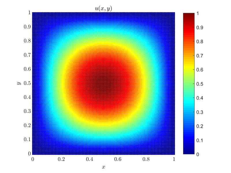
It is fitting that examples start with a simple case, and we will gradually make our way towards more complicated cases with different domain shapes, boundary conditions and approximation types. Consider the solution of the 2D Poisson equation on a unit square with Dirichlet boundary conditions\[ \begin{align*} \Delta u &= f &&\text{in } \Omega, \\ u &= 0 &&\text{on } \partial \Omega, \end{align*} \] where $u(x,y)$ is the solution to the problem, $\Omega = [0, 1] \times [0, 1]$ and in the case we will consider $f(x,y) = -2\pi^2\sin(\pi x)\sin(\pi y)$, as it makes for a simple solution $u(x,y) = \sin(\pi x)\sin(\pi y)$.
First, we construct our domain and discretize it, then find support (neighborhood) for each node.
1 BoxShape<Vec2d> box(0.0, 1.0);
2 double dx = 0.01;
3 DomainDiscretization<Vec2d> domain = box.discretizeWithStep(dx);
4
5 int N = domain.size();
6 domain.findSupport(FindClosest(9));
We constructed a box shape, discretized it with a constant step dx (both inside and the boundary) and choose the closest 9 nodes of each node as its support. The next step is to construct our approximation engine. Simply put, approximation engines are classes responsible for computing shape functions for given operator and points. While many different setups are supported in Medusa we will start off simple, with an approximation that reproduces standard Finite Difference method.
1 int m = 2
2 WLS<Monomials<Vec2d>, NoWeight<Vec2d>, ScaleToFarthest> wls(Monomials<Vec2d>::tensorBasis(m));
We constructed a WLS engine using monomial tensor basis of order 2. Finally, we write the equations for our problem by directly translating the mathematical formulation above into code.
1 for (int i : domain.interior()) {
2     double x = domain.pos(i, 0);
3     double y = domain.pos(i, 1);
4     op.lap(i) = -2*PI*PI*std::sin(PI*x)*std::sin(PI*y);
5 }
6 for (int i : domain.boundary()) {
7     op.value(i) = 0.0;
8 }
Here is the plot of the solution $u(x, y)$.
The whole example can be found as poisson_dirichlet_2D.cpp along with the plot script that can be run by Matlab or Octave poisson_dirichlet_2D.m. Same goes for similar cases solved in 1D and 3D and their respective plot scripts.
Mixed boundary conditions
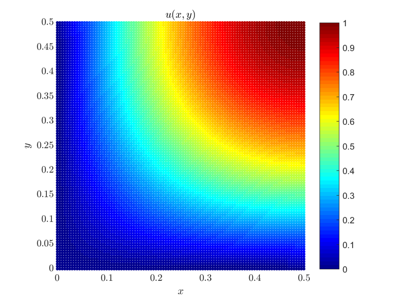
We can obtain the solution to the above problem by solving it on just a quarter of the original domain and using mixed boundary conditions. By using Dirichlet boundary conditions on the bottom and the left side of the square domain, and Neumann boundary conditions on the right and upper side of the domain we are effectively solving the same problem but on a quarter of the domain. Our problem is now\[ \begin{align*} \Delta u &= f &&\text{in } \Omega, \\ u &= 0 &&\text{on } \partial \Omega_1 \cup \partial \Omega_3,\\ \frac{du}{d \b{\hat{n}}} &= 0 &&\text{on } \partial \Omega_2 \cup \partial \Omega_4 \end{align*} \]
Where $\partial \Omega_1$, $\partial \Omega_2$, $\partial \Omega_3$ and $\partial \Omega_4$ are left, right, bottom and top boundary respectively. The domain is $\Omega = [0, 0.5] \times [0, 0.5]$, and $\frac{du}{d \b{\hat{n}}}$ is the normal derivative (on the boundary).
When constructing approximation engines, there are a lot of different options, you can choose between different basis functions, weights, scale functions and each setup comes with its advantages and disadvantages. Some might work for certain problems and some might not. When writing the examples we tried to present the reader with as many different options as possible.
Let us solve the problem using Gaussian RBF (Radial Basis Functions) instead of Monomials:
1     // shape = 30
2     // m = 9
3     WLS<Gaussians<Vec2d>, NoWeight<Vec2d>, ScaleToFarthest,
4             Eigen::LLT<Eigen::MatrixXd>> wls({9, 30});
While the case is the same for the nodes inside the domain, we need to change the boundary conditions:
 1     int BOTTOM = -3;
 2     int TOP = -4;
 3     int LEFT = -1;
 4     int RIGHT = -2;
 5
 6     for (int i : (domain.types() == LEFT) + (domain.types() == BOTTOM)) {
 7         op.value(i) = 0.0;  // Dirichlet boundary conditions on the left and bottom edge of the box
 8     }
 9     for (int i : (domain.types() == TOP) + (domain.types() == RIGHT)) {
10         // Neumann boundary conditions on upper and right edge of the box
11         op.neumann(i, domain.normal(i)) = 0.0;
12     }
When solving a PDE implicitly a system of equations needs to be solved to obtain the solution. For this, we use Eigen.
1     Eigen::BiCGSTAB<decltype(M), Eigen::IncompleteLUT<double>> solver;
2     solver.compute(M);
3     ScalarFieldd u = solver.solve(rhs);
Matrix M and rhs are the sparse matrix and vector in which we wrote (with the help of Medusa) the system of equations that when solved gives us an approximate solution of our problem. We solve the system using an Eigen linear equation solver, in this case, the BiCGStab algorithm with ILUT preconditioning. The solution is plotted below:
The whole example can be found as poisson_mixed_2D.cpp along with the plot script that can be run by Matlab or Octave poisson_mixed_2D.m. Similar examples such as mixed boundary conditions on a circular domain, mixed boundary conditions on an irregular domain and a solution to a similar problem using monomial augmentation of radial basis functions can be found here.
Full Neumann boundary conditions
When solving the Navier-Stokes equation with Explicit Pressure correction, a Poisson's equation with full Neumann boundary conditions needs to be solved. In order for this type of problem to be solved, it needs to satisfy the compatibility condition. Inside the domain we still have:
$$ \Delta u = f $$
The Poisson equation has a solution for the requisite function $u(x,y)$, when the integral of the source function $f(x,y)$ over our domain needs to be equal to the net flow rate, that is expressed by the boundary integral of the normal derivative of $u(x,y)$. In mathematical formulation, for our 2D case:
$$ \int_{\Omega} f(x,y) dxdy = \int_{\partial \Omega} \frac{du}{d \b{\hat{n}}} dl $$
Where again $\Omega$ is our domain, $\partial \Omega$ is the boundary of our domain, $dl$ is the differential arc length along the boundary. When the compatibility condition is met, the Poisson equation has a solution that can be determined up to an arbitrary constant. To obtain only one solution another constraint needs to be implemented. One option is to select a node and set it to a constant, e.g. p(0, 0) = 0, however much more stable approach is to enforce solution with an additional condition, also referred to as a regularization:
$$ \int_{\Omega }^{{}}{u(x,y)d}\Omega = 0 $$
On our unit square domain, $\Omega = [0, 1] \times [0, 1]$ an example case that satisfies the compatibility condition would be:
 1     for (int i : domain.interior()) {
 2         op.lap(i) = 2;
 3     }
 4
 5     int BOTTOM = -3;
 6     int TOP = -4;
 7     int LEFT = -1;
 8     int RIGHT = -2;
 9
10     for (int i : (domain.types() == LEFT)) {
11         op.der1(i, 0) = 0.0;
12     }
13     for (int i : (domain.types() == RIGHT)) {
14         op.der1(i, 0) = 1.0;
15     }
16     for (int i : (domain.types() == BOTTOM)) {
17         op.der1(i, 1) = 0.0;
18     }
19     for (int i : (domain.types() == TOP)) {
20         op.der1(i, 1) = 1.0;
21     }
Which is simply, $\Delta u = 2$ inside $\Omega$ while $\frac{du}{d \b{\hat{n}}} = 1$ on top and right boundary and $\frac{du}{d \b{\hat{n}}} = 0$ on the other two. With a little mental math we see that the compatibility condition is met, $2 * 1 = 0 + 1 + 0 + 1$. With that out of the way let us see how we implement regularization:
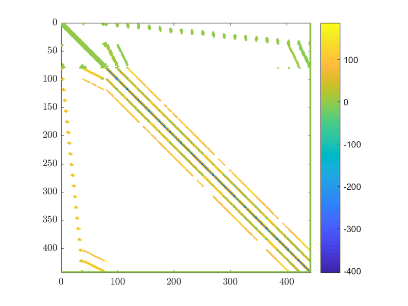
Well the idea add another line and column to matrix M holding the shape function s, and enforce the condition. We do this by adding a Lagrange multiplier $\alpha$:
$$ \left[ \begin{matrix} {{M}_{11}} & .. & {{M}_{1n}} & 1 \\ .. & .. & .. & 1 \\ {{M}_{n1}} & ... & {{M}_{nn}} & 1 \\ 1 & 1 & 1 & 0 \\ \end{matrix} \right]\left[ \begin{matrix} {{u}_{1}} \\ ... \\ {{u}_{n}} \\ \alpha \\ \end{matrix} \right]=\left[ \begin{matrix} rhs_1 \\ ... \\ rhs_n \\ 0 \\ \end{matrix} \right] $$
When the problem is well-posed $\alpha$ should be equal to zero, or at least very close. Let us fill our matrix M:
1     // regularization
2     // set the last row and column of the matrix
3     for (int i = 0; i < N; ++i) {
4         M.coeffRef(N, i) = 1;
5         M.coeffRef(i, N) = 1;
6     }
7     // set the sum of all values
8     rhs[N] = 0.0;
If we take a look at the matrix we will see the extra row and column that enforce our constraint. They should be the last column and the last row of the matrix:
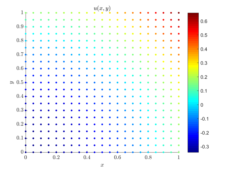
With this done we can solve the problem, just as we did in the examples above.
For $dx = 0.05$ we get $\alpha = -1.03846 \cdot 10^{-13}$, which is expected from a valid solution.
The whole example can be found as poisson_neumann_2D.cpp along with the plot script that can be run by Matlab or Octave poisson_neumann_2D.m.
3D model case
A 3D domain triceratops.h5 was created from the Mathematica's triceratops model. The point coordinates can be imported to medusa and used as a domain. In the example given in triceratops.cpp
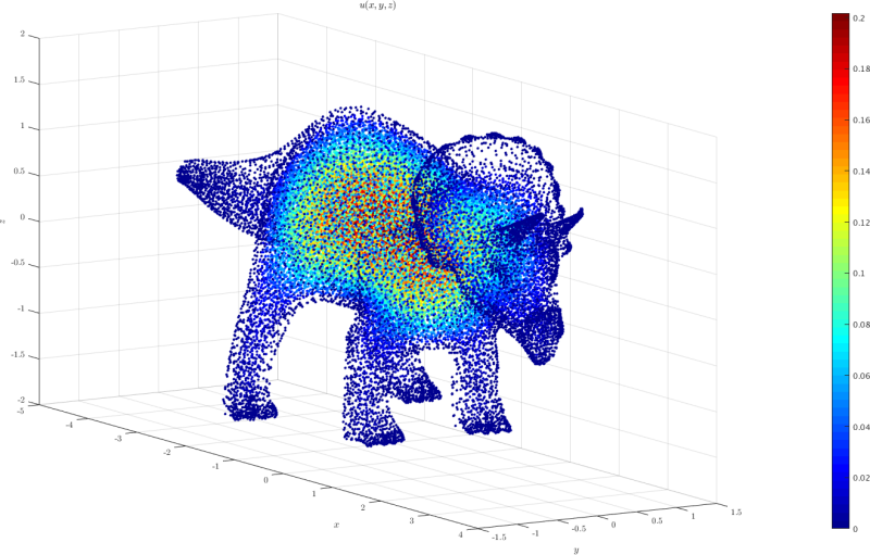
the equation $-\nabla^u = 1$ with $u=0$ on the boundary is solved.
The plot of the solution obtained using triceratops.m is shown below:
Convergence rate - including high order solution
Assume a $d$-dimensional Poisson problem with mixed boundary conditions.
\( \begin{align*} \nabla ^2 u(\boldsymbol x) &= -d \pi ^2 \prod_{i=1} ^d \sin(\pi x_i) \qquad &&\text{in } \Omega, \\ u(\boldsymbol x) &= \prod _{i = 1} ^d \sin(\pi x_i) \qquad && \text{on } \Gamma_d,\\ \frac{\partial u}{\partial \boldsymbol n}(\boldsymbol x) &= \pi \sum_{i=1}^d n_i \cos(\pi x_i) \prod_{j\neq i} \sin(\pi x_j) \qquad && \text{on } \Gamma_n, \end{align*} \)
where $n_i$ are components of the unit normal vector $\boldsymbol n$, $\Omega$ is a $d$-dimensional ball with origin at $\boldsymbol x = \boldsymbol{1} \boldsymbol{/} \boldsymbol{2}$ and radius $r = 1/2$, and $\Gamma_d$, $\Gamma_n$ are left and right halves of the boundary, respectively\[ \begin{align*} \Omega &= \left\{ \boldsymbol x, \ \left\|\boldsymbol x - \boldsymbol{\frac 1 2}\right\| < \frac 1 2 \right\}, \\ \Gamma_d &= \left \{ \boldsymbol x \in \partial \Omega,\boldsymbol x_1 < \frac 1 2 \right \}, \\ \Gamma_n &= \left \{ \boldsymbol x \in \partial \Omega,\boldsymbol x_1 \geq \frac 1 2 \right \}. \end{align*} \]
Solution of the above case is $u(\boldsymbol x) = \prod _{i = 1} ^d \sin(\pi x_i)$, allowing us to validate the numerically obtained solution $u_h$.
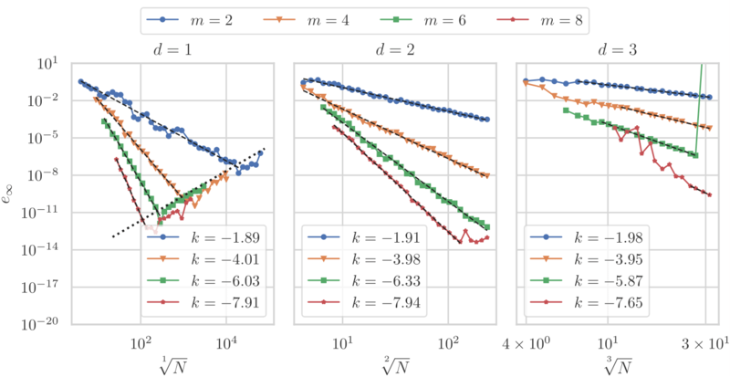
Numerical results are computed using RBF-FD with PHS radial basis function $\phi(r) = r^3$ and monomial augmentation - thus control over the method order is enabled. Radial function was kept same for all cases, however, various orders of monomial augmentation were tested. Solution to the problem is obtained using monomials up to and including degree $m$, for $m \in \left \{2, 4, 6, 8 \right \}$.
Figure above shows the $e_\infty$ error for $d=1$, $d=2$, and $d=3$ dimensions. The span of the horizontal axis is chosen in such a way that the total number of nodes in the largest case was around $N = 10^5$ in all dimensions. The observed convergence rates are independent of domain dimension and match the predicted order $O(h^m)$. All of the plots in $d=1$ case and $m=8$ sub-case of $d=2$ case eventually diverge due to the errors in finite precision arithmetic. The dotted line in $d=1$ case shows the $\varepsilon/h^2$ line, where $\varepsilon \approx 2.22 \cdot 10^{-16}$.
Higher dimensional space
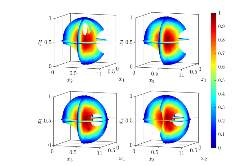
We now demonstrate a solution to a Poisson problem in a 4-dimensional irregular domain. The irregular domain $\Omega$ is defined as $\Omega = B_ 0 \setminus (B_ 1 \cup B_ 2 \cup B_ 3)$, where
\( \begin{align*} B_ 0 &= \left \{\boldsymbol x \in \R^4, \ \left\|\boldsymbol x - \boldsymbol{\frac 1 2}\right\| < \frac 1 2 \right \}, \\ B_ 1 &= \left \{\boldsymbol x \in \R^4, \ \left\|\boldsymbol x - \left(\frac 1 2, 1, \frac 1 2, \frac 1 2\right)\right\| \le \frac 1 4 \right \}, \\ B_ 2 &= \left \{\boldsymbol x \in \R^4, \ \left\|\boldsymbol x - \boldsymbol{0}\right\| \le \frac{13}{16} \right \} \text{ and} \\ B_ 3 &= \left \{\boldsymbol x \in \R^4, \ \left\|\boldsymbol x - \left(\frac 1 2, \frac 1 2, \frac 3 4, \frac 1 2\right)\right\| \le \frac 1 8 \right \} \end{align*} \)
are balls in $\R^4$.
Dirichlet and Neumann boundary conditions are defined similarly to before, i.e. $\Gamma_d$ is the left half and $\Gamma_n$ is the right half of $\partial\Omega$. Additionally the boundary of the smallest ball $\partial B_ 3$ is added to Dirichlet boundary
\( \begin{align*} \Gamma_d &= \left \{ \boldsymbol x\in \partial \Omega, x_1 < \frac 1 2 \right \} \cup \partial B_3 ,\\ \Gamma_n &= \left \{ \boldsymbol x\in \partial \Omega, x_1 \geq \frac 1 2 \right \} \setminus \partial B_ 3. \end{align*} \)
Numerical solution $u_h$ was obtained using RBF-FD with PHS $\phi (r) = r^3$ augmented with polynomials of degree $m=2$
Figure below shows the numerically obtained solution. Four three-dimensional slices are shown, defined by setting one coordinate to $x_i = 1/2$. Modified Sheppard's interpolation algorithm was used to interpolate the solution to an intermediate grid, used for plotting the slices.
Go back to Examples.
