Difference between revisions of "Relaxation of the nodal distribution"
(Created page with "''TODO(Uduh): rewrite'' To construct stable and reliable shape functions the support domains need to be non-degenerated [1], i.e. the distances between support nodes have to...") |
E6WikiAdmin (talk | contribs) |
||
| (4 intermediate revisions by 2 users not shown) | |||
| Line 1: | Line 1: | ||
| − | + | {{Box-round|title= Related papers | | |
| − | To construct stable and reliable shape functions the support domains need to be non-degenerated | + | [https://e6.ijs.si/ParallelAndDistributedSystems/publications/31107623.pdf J. Slak, G. Kosec; Refined meshless local strong form solution of Cauchy-Navier equation on an irregular domain, Engineering analysis with boundary elements, vol. 100, 2019] |
| + | |||
| + | [https://e6.ijs.si/ParallelAndDistributedSystems/publications/29512743.pdf G. Kosec; A local numerical solution of a fluid-flow problem on an irregular domain, Advances in engineering software, vol. 120, 2018 [DOI: 10.1016/j.advengsoft.2016.05.010]] | ||
| + | }} | ||
| + | |||
| + | To construct stable and reliable shape functions the support domains need to be non-degenerated <ref name="LeeLocal">Lee CK, Liu X, Fan SC. Local muliquadric approximation for solving boundary value problems. Comput Mech. 2003;30:395-409.</ref>, i.e. the distances between support nodes have to be balanced. Naturally, this condition is fulfilled in regular nodal distributions, but when working with complex geometries, the nodes have to be positioned accordingly. There are different algorithms designed to optimally fill the domain with different shapes <ref name="LohnerGeneral">Löhner R, Oñate E. A general advancing front technique for filling space with arbitrary objects. Int J Numer Meth Eng. 2004;61:1977-91.</ref><ref name="LiuNode">Liu Y, Nie Y, Zhang W, Wang L. Node placement method by bubble simulation and its application. CMES-Comp Model Eng. 2010;55:89.</ref>, see [[Positioning of computational nodes]] for our algorithms. Here, an intrinsic feature of the MLSM is used to take care of that problem. The goal is to minimize the overall support domain degeneration in order to attain stable numerical solution. In other words, a global optimization problem with the overall deformation of the local support domains acting as the cost function is tackled. We seek the global minimum by a local iterative approach. In each iteration, the computational nodes are translated according to the local derivative of the potential | ||
\begin{equation} | \begin{equation} | ||
| − | \delta \b{p}\left( \b{p} \right)=-\sigma_{k}\sum\limits_{ | + | \delta \b{p}\left( \b{p} \right)=-\sigma_{k}\sum\limits_{i=1}^{n}{\nabla }V\left( \b{p}-\b{p}_i \right) |
\end{equation} | \end{equation} | ||
| − | where $V, n, \delta \b{p}, \b{p}_{ | + | where $V, n, \delta \b{p}, \b{p}_{i}$ and $\sigma_{k}$ stand for the potential, number of support nodes, offset of the node, position of i-th support node and relaxation parameter, respectively. After offsets in all nodes are computed, the nodes are repositioned as |
$\b{p}\leftarrow \b{p}+\delta \b{p}\left( \b{p} \right)$. | $\b{p}\leftarrow \b{p}+\delta \b{p}\left( \b{p} \right)$. | ||
Presented iterative process procedure begins with positioning of boundary nodes, which is considered as the definition of the domain, and then followed by the positioning of internal nodes. | Presented iterative process procedure begins with positioning of boundary nodes, which is considered as the definition of the domain, and then followed by the positioning of internal nodes. | ||
| − | The BasicRelax | + | The <code>BasicRelax</code> engine supports two call types: |
| − | * with supplied distribution function relax(func), where it tries to satisfy the user supplied nodal density function. This can be achieved only when there is the total number of domain nodes the same as integral of density function over the domain. If there is too much nodes a volatile relax might occur. If there is not enough nodes the relax might become lazy. The best use of this mode is in combination with | + | * with supplied distribution function <code>relax(domain, func)</code>, where it tries to satisfy the user supplied nodal density function <code>func</code>. This can be achieved only when there is the total number of domain nodes the same as integral of density function over the domain. If there is too much nodes a volatile relax might occur. If there is not enough nodes the relax might become lazy. The best use of this mode is in combination with <code>GeneralFill</code> and/or <code>GeneralSurfaceFill</code>. |
* without distribution, where nodes always move towards less populated area. The relax magnitude is simply determined from Annealing factor and distance to the closest node. A simple and stable approach, however, note that this relax always converges towards uniformly distributed nodes. | * without distribution, where nodes always move towards less populated area. The relax magnitude is simply determined from Annealing factor and distance to the closest node. A simple and stable approach, however, note that this relax always converges towards uniformly distributed nodes. | ||
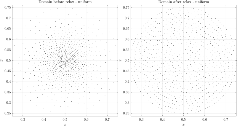
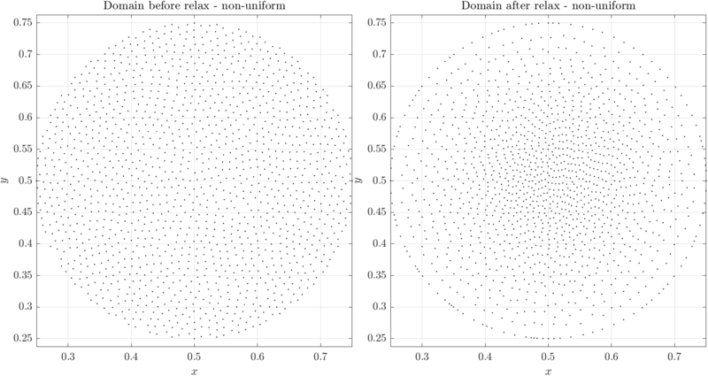
| − | Example of filling and relaxing 2D domain can be found in below code snippet and | + | Example of filling and relaxing a 2D domain can be found in below code snippet and Figures. Note the difference between relax without supplied distribution (<xr id="fig:relax_uniform"/>) and with supplied distribution (<xr id="fig:relax_non-uniform"/>). These examples are extreme, relaxation is usually used to convert an almost desirable node distribution into a desirable node distribution. |
More examples can be found in main repository under tests. | More examples can be found in main repository under tests. | ||
<syntaxhighlight lang="c++" line> | <syntaxhighlight lang="c++" line> | ||
| − | + | // Define domain shape. | |
| − | + | double r = 0.25; | |
| − | + | BallShape<Vec2d> bs({0.5, 0.5}, r); | |
| − | |||
| − | |||
| − | |||
| − | |||
| − | |||
| − | |||
| − | + | // Fill domain disretization with h. | |
| − | + | auto h = [](Vec2d p){ | |
| + | return (0.005 + (p[0] - 0.5) * (p[0] - 0.5) / 2 + (p[1] - 0.5) * (p[1] - 0.5) / 2); | ||
| + | }; | ||
| + | DomainDiscretization<Vec2d> domain = bs.discretizeBoundaryWithDensity(h); | ||
| + | GeneralFill<Vec2d> gf; | ||
| + | gf(domain, h); | ||
| − | + | // Relax domain to uniform distribution. | |
| − | + | BasicRelax relax; | |
| + | relax.iterations(1000).initialHeat(1).finalHeat(0).boundaryProjectionThreshold(0.75) | ||
| + | .projectionType(BasicRelax::PROJECT_IN_DIRECTION).numNeighbours(5); | ||
| + | relax(domain); | ||
</syntaxhighlight> | </syntaxhighlight> | ||
| + | <figure id="fig:relax_uniform"> | ||
| + | [[File:relax_uniform.png|thumb|center|800px|<caption> Relaxation of a non-uniform node distribution to a uniform node distribution. </caption>]] | ||
| + | </figure> | ||
| − | [[File: | + | <figure id="fig:relax_non-uniform"> |
| − | + | [[File:relax_non-uniform.png|thumb|center|800px|<caption> Relaxation of a uniform node distribution to a non-uniform node distribution. </caption>]] | |
| − | + | </figure> | |
| − | |||
| − | |||
| − | |||
| − | + | =References= | |
| + | <references/> | ||
Latest revision as of 20:21, 22 October 2022
Related papers
To construct stable and reliable shape functions the support domains need to be non-degenerated [1], i.e. the distances between support nodes have to be balanced. Naturally, this condition is fulfilled in regular nodal distributions, but when working with complex geometries, the nodes have to be positioned accordingly. There are different algorithms designed to optimally fill the domain with different shapes [2][3], see Positioning of computational nodes for our algorithms. Here, an intrinsic feature of the MLSM is used to take care of that problem. The goal is to minimize the overall support domain degeneration in order to attain stable numerical solution. In other words, a global optimization problem with the overall deformation of the local support domains acting as the cost function is tackled. We seek the global minimum by a local iterative approach. In each iteration, the computational nodes are translated according to the local derivative of the potential
\begin{equation}
\delta \b{p}\left( \b{p} \right)=-\sigma_{k}\sum\limits_{i=1}^{n}{\nabla }V\left( \b{p}-\b{p}_i \right)
\end{equation}
where $V, n, \delta \b{p}, \b{p}_{i}$ and $\sigma_{k}$ stand for the potential, number of support nodes, offset of the node, position of i-th support node and relaxation parameter, respectively. After offsets in all nodes are computed, the nodes are repositioned as
$\b{p}\leftarrow \b{p}+\delta \b{p}\left( \b{p} \right)$.
Presented iterative process procedure begins with positioning of boundary nodes, which is considered as the definition of the domain, and then followed by the positioning of internal nodes.
The BasicRelax engine supports two call types:
- with supplied distribution function
relax(domain, func), where it tries to satisfy the user supplied nodal density functionfunc. This can be achieved only when there is the total number of domain nodes the same as integral of density function over the domain. If there is too much nodes a volatile relax might occur. If there is not enough nodes the relax might become lazy. The best use of this mode is in combination withGeneralFilland/orGeneralSurfaceFill. - without distribution, where nodes always move towards less populated area. The relax magnitude is simply determined from Annealing factor and distance to the closest node. A simple and stable approach, however, note that this relax always converges towards uniformly distributed nodes.
Example of filling and relaxing a 2D domain can be found in below code snippet and Figures. Note the difference between relax without supplied distribution (Figure 1) and with supplied distribution (Figure 2). These examples are extreme, relaxation is usually used to convert an almost desirable node distribution into a desirable node distribution. More examples can be found in main repository under tests.
 1 // Define domain shape.
 2 double r = 0.25;
 3 BallShape<Vec2d> bs({0.5, 0.5}, r);
 4
 5 // Fill domain disretization with h.
 6 auto h = [](Vec2d p){
 7     return (0.005 + (p[0] - 0.5) * (p[0] - 0.5) / 2 + (p[1] - 0.5) * (p[1] - 0.5) / 2);
 8 };
 9 DomainDiscretization<Vec2d> domain = bs.discretizeBoundaryWithDensity(h);
10 GeneralFill<Vec2d> gf;
11 gf(domain, h);
12
13 // Relax domain to uniform distribution.
14 BasicRelax relax;
15 relax.iterations(1000).initialHeat(1).finalHeat(0).boundaryProjectionThreshold(0.75)
16      .projectionType(BasicRelax::PROJECT_IN_DIRECTION).numNeighbours(5);
17 relax(domain);
References
- ↑ Lee CK, Liu X, Fan SC. Local muliquadric approximation for solving boundary value problems. Comput Mech. 2003;30:395-409.
- ↑ Löhner R, Oñate E. A general advancing front technique for filling space with arbitrary objects. Int J Numer Meth Eng. 2004;61:1977-91.
- ↑ Liu Y, Nie Y, Zhang W, Wang L. Node placement method by bubble simulation and its application. CMES-Comp Model Eng. 2010;55:89.

