Difference between revisions of "Heart rate variability detection"
(Created page with "We used MLS and WLS aproximation to extract heart rate variability from a wearable ECG sensor. [http://www-e6.ijs.si/ParallelAndDistributedSystems/MeshlessMachine/technical_do...") |
(→Fine local search) |
||
| (5 intermediate revisions by 3 users not shown) | |||
| Line 1: | Line 1: | ||
We used MLS and WLS aproximation to extract heart rate variability from a wearable ECG sensor. | We used MLS and WLS aproximation to extract heart rate variability from a wearable ECG sensor. | ||
| − | |||
| − | |||
The code can be found in <syntaxhighlight lang="bash" inline> /EKG/detect.cpp </syntaxhighlight>. | The code can be found in <syntaxhighlight lang="bash" inline> /EKG/detect.cpp </syntaxhighlight>. | ||
| Line 13: | Line 11: | ||
=Detection of heart rate variability<br>from a wearable differential ECG device= | =Detection of heart rate variability<br>from a wearable differential ECG device= | ||
| − | [mailto:jure.slak@ | + | [mailto:jure.slak@ijs.si Jure Slak], [mailto:gregor.kosec@ijs.si Gregor Kosec], |
Jožef Stefan Insitute, Department of Communication Systems, Ljubljana. | Jožef Stefan Insitute, Department of Communication Systems, Ljubljana. | ||
| Line 142: | Line 140: | ||
approximation is valid only as long as the evaluation point is close to the | approximation is valid only as long as the evaluation point is close to the | ||
$t_0$. | $t_0$. | ||
| − | A more general approach is a [[ | + | A more general approach is a [[Weighted Least Squares (WLS)|Moving Least Square (MLS)]] approximation, where |
coefficients $\alpha$ are not spatially independent any more, but are recomputed | coefficients $\alpha$ are not spatially independent any more, but are recomputed | ||
for each evaluation point. Naturally, such an approach is way more expensive, | for each evaluation point. Naturally, such an approach is way more expensive, | ||
| Line 154: | Line 152: | ||
with measurements taken at points $ \{-14, \ldots, 24\} $.</caption>]] | with measurements taken at points $ \{-14, \ldots, 24\} $.</caption>]] | ||
</figure> | </figure> | ||
| + | |||
| + | The task of finding the minimal value of the first derivative is equivalent to | ||
| + | the task of finding the zero of the second derivative. This zero will be our local | ||
| + | approximation $t_L$ of the beat time, $\hat{f}''(t_L) = 0$. | ||
| + | Therefore an approximation function with a non constant second derivative, | ||
| + | i.e. approximation function with a | ||
| + | minimal 3rd order monomial basis, is constructed. The most straightforward | ||
| + | approach to find its root is the simple bisection. Bisection requires initial | ||
| + | low and high bounds that can be estimated from characteristic point $t_G$ | ||
| + | provided by the global method. Using the fact that the QRS intervals last | ||
| + | approximately $\Delta t_{\text{QRS}}= 0.1 s$, we can seek for the root of the second | ||
| + | derivative on an interval $[t_G - \Delta t_{\text{QRS}}/2, t_G + \Delta | ||
| + | t_{\text{QRS}}/2]$, and at given sample rate this translates to the search | ||
| + | interval of two sample points away from $t_G$ in each direction. | ||
| + | |||
| + | ==HRV calculation and error estimation== | ||
| + | Given sampled heartbeat, the fine local search produces the vector of $\ell+1$ detected times | ||
| + | $\boldsymbol{t_L} := (t_{L,i})_{i=1}^{\ell+1}$ of the RS slopes. Their successive | ||
| + | differences represent a vector $\boldsymbol{\hat{r}}$ of detected beat to beat times, | ||
| + | the durations of RR intervals. | ||
| + | \[ \boldsymbol{\hat{r}} = (\hat{r}_{i})_{i=1}^\ell, \quad \hat{r}_i = t_{L,i+1} - t_{L,i} \] | ||
| + | Let $\boldsymbol{r}$ be the vector of (usually unknown) actual beat to beat times. Then the | ||
| + | heart rate variability (HRV) $h$ is defined as | ||
| + | \[ h := \text{std}(\boldsymbol{r}) = \sqrt{\frac{1}{\ell}\sum_{i=1}^{\ell} (r_i - \bar{r})^2}, \] | ||
| + | where $\bar{r}$ stands for the average beat to beat time, $\bar{r} = | ||
| + | \sum_{i=1}^\ell r_i / \ell$. The HRV estimation $\hat{h}$ is calculated as the | ||
| + | standard deviation of the detected times $\boldsymbol{\hat{r}}$. | ||
| + | |||
| + | In the following analyses the actual vector $\boldsymbol{r}$ will be known, since the | ||
| + | synthesized heartbeat will be analysed. The most obvious error measures are the | ||
| + | absolute error of HRV, $e_{h} = |\hat{h} - h|$ and the absolute error of the | ||
| + | average heart beat $e_{\bar{r}} = |\bar{\hat{r}} - \bar{r}|$. Using the vector | ||
| + | of errors $\boldsymbol{e} = |\boldsymbol{r} -\boldsymbol{\hat{r}}|$ the average error $e_a = \sum e_i | ||
| + | / \ell$ and the maximal error $e_M = \max(\boldsymbol{e})$ can be assessed. | ||
| + | |||
| + | =Results and discussion= | ||
| + | |||
| + | ==Approximation set-up== | ||
| + | |||
| + | <figure id="fig:results"> | ||
| + | [[File:results.png|600px|thumb|upright=2|alt= Beat graph|<caption> Subfigures $\begin{bmatrix} a & b & ,& c & d \end{bmatrix}$. <br> | ||
| + | Subfigure a. Sufficiently small support implies interpolation, | ||
| + | making weight function useless and MLS equal to WLS. <br> | ||
| + | Subfigure b. MLS and WLS differ when approximating with a low order polynomial. <br> | ||
| + | Subfigure c. MLS and WLS match when approximating with a high order polynomial.<br> | ||
| + | Sunfigure d. Expected bad behaviour with too many support points and a low order approximation.</caption>]] | ||
| + | </figure> | ||
| + | |||
| + | In first step the approximation free parameters, i.e. weight function, support | ||
| + | size, and number of basis functions, have to be assessed. A single heartbeat is | ||
| + | extracted and approximated with all possible combinations of basis functions | ||
| + | with orders from $2$ to $10$ and symmetric supports of sizes from $3$ to $15$ using both | ||
| + | WLS and MLS. An global algorithm described in previous section was used | ||
| + | to produce the initial guesses. For demonstration four sample cases are | ||
| + | presented. The weight function was the same in all four cases, a Gaussian | ||
| + | distribution with $\mu = t_G$ and $\sigma = m/4$, which makes sure that all | ||
| + | support points are taken into account, but the central ones are more important. | ||
| + | |||
| + | The simplest case is when the support size is the same as number of basis | ||
| + | functions resulting in an interpolation. In this case, the weight function is | ||
| + | not important, making WLS and MLS entirely equivalent as seen in | ||
| + | <xr id="fig:results"/>a. | ||
| + | |||
| + | In case of small support and small order of monomial basis WLS performs worse | ||
| + | than MLS and the approaches differ significantly. However, as we increase the | ||
| + | order of the polynomial basis the difference within the bisection interval | ||
| + | becomes negligible. This transition can be observed in <xr id="fig:results"/>b and <xr id="fig:results"/>c. | ||
| + | |||
| + | As predicted, the support size is important. Both methods perform badly when | ||
| + | too many surrounding measurements are taken into account while still using a low | ||
| + | order polynomial approximation. Note that in <xr id="fig:results"/>d the initial | ||
| + | guess is barely improved and the beat shape is skewed away from the RS drop. | ||
| + | |||
| + | The conclusion is, that for our purposes MLS approximation is unnecessary, as | ||
| + | WLS provides good enough results, when used appropriately. Further analysis | ||
| + | to determine the best choice of parameters $m$ and $n$ is presented later. | ||
| + | |||
| + | |||
| + | ==Computational complexity== | ||
| + | The presented algorithm is a streaming algorithm, requiring a buffer to store | ||
| + | the current beat in the signal. Let $b$ be the number of measurements per | ||
| + | beat, stored in a buffer of length $b$. The global part of the algorithm | ||
| + | makes $O(b)$ operations, being a simple local search. The local part is | ||
| + | more expensive. First a $n \times m$ matrix is constructed in $O(mn)$ | ||
| + | and the right hand side vector is copied from the buffer. The system is then | ||
| + | solved using SVD decomposition in $O(mn^2+n^3)$ . Note that as $m = | ||
| + | O(n)$, this step takes $O(n^3)$. The minimal first derivative is found | ||
| + | using bisection. To achieve tolerance $\varepsilon$, | ||
| + | $\lceil\log_2(1/\varepsilon)\rceil$ function evaluations are needed, each | ||
| + | costing $O(m)$ operations. Total time complexity is therefore equal to | ||
| + | $O(b + n^3 + m\log(1/\varepsilon))$. Note, that using MLS would require | ||
| + | $O(n^3)$ for each function evaluation, resulting in a significantly worse | ||
| + | time complexity of $O(b+n^3\log_2(1/\varepsilon)))$. The calculation of | ||
| + | average and variance is done later, after the wanted amount of signal has | ||
| + | already been analysed. | ||
| + | |||
| + | In practice the algorithm executes very fast, using typical values $b = | ||
| + | 150$, $m=6$, $n=11$ and $\varepsilon = 10^{-10}$ it runs | ||
| + | approximately $0.27$ s to analyze $1000$ heartbeats ($\approx 10^5$ data | ||
| + | points). The algorithm was compiled from C++ source code using | ||
| + | <syntaxhighlight lang="bash" inline> g++5.3.0</syntaxhighlight> with <syntaxhighlight lang="bash" inline> -O2 </syntaxhighlight> flag and run on | ||
| + | an <tt>Intel(R) Core(TM) i7-4700MQ</tt> processor. | ||
| + | |||
| + | ==Simulated heartbeat with known variability== | ||
| + | |||
| + | <figure id="fig:variabilityscatter"> | ||
| + | [[File:variabilityscatter.png|600px|thumb|upright=2|alt= Generated beat to beat times and their global detection|<caption>Generated beat to beat times and their global detection.</caption>]] | ||
| + | </figure> | ||
| + | |||
| + | The first set of tests for the presented method was performed using a simulated | ||
| + | heartbeat. A single real heartbeat was taken and then replicated thousand | ||
| + | times, each time shifted by a random offset $T$, distributed normally | ||
| + | around zero, $T \sim \mathcal{N}(0, \sigma^2)$, with $\sigma = | ||
| + | \frac{1}{2\nu} = \frac{1}{2} \Delta t$. This means that a decent amount of | ||
| + | measurements will be more than $\Delta t$ apart, a difference that must be | ||
| + | detected by global search for method to work. However, around half of the | ||
| + | measurements are less than $\Delta t$ apart, forming suitable ground for | ||
| + | testing the precision of the local search. At given sample frequency, | ||
| + | $\sigma$ equals $4.167 ms$. | ||
| + | |||
| + | The generated beat to beat times, coarsely detected and finely detected times | ||
| + | are presented in <xr id="fig:variabilityscatter"/>. | ||
| + | |||
| + | Beat to beat time precision is significantly improved by the local search. | ||
| + | As seen in <xr id="fig:variabilityhist"/>, the distributions of generated and detected | ||
| + | heart beats match very well. | ||
| + | |||
| + | <figure id="fig:variabilityhist"> | ||
| + | [[File:variabilityhist.png|600px|thumb|center|upright=2|alt= Generated RRI times and their global detection|<caption>Generated RRI times and their global detection. | ||
| + | The middle two coarse detection columns continue off the chart, but are not shown completely for clarity.</caption>]] | ||
| + | </figure> | ||
| + | |||
| + | Results of RRI and HRV detection by global and local search are presented in | ||
| + | Table 1. The generated times were taken as precise and the | ||
| + | algorithm was run to produce global and local approximations. Then the average | ||
| + | RRI time and HRV were calculated for each data set separately. The average RRI | ||
| + | time is estimated very well with both methods, but the precision of the global | ||
| + | method is not satisfactory when measuring heart rate variability. The precision | ||
| + | is significantly improved using the local search. A chart showing the average | ||
| + | error of the detected times is shown in <xr id="fig:allerrs"/>. It can be seen | ||
| + | that MLS performs better on average, but WLS is very close and this loss of | ||
| + | precision is a reasonable tradeoff. | ||
| + | |||
| + | <figure id="fig:allerrs"> | ||
| + | [[File:allerrs.png|600px|thumb|center|upright=2|alt= Comparison of WLS and MLS errors|<caption> Comparison of WLS and MLS errors using different orders and | ||
| + | support sizes.</caption>]] | ||
| + | </figure> | ||
| + | |||
| + | The red values in <xr id="fig:allerrs"/> indicate invalid region, having more basis functions than support points. | ||
| + | Both MLS and WLS have the same region of validity, being precise in the predicted regime. | ||
| + | For very high order approximation the condition number of the matrix becomes critical | ||
| + | and the method is unstable, which explains the loss of precision for orders larger than $12$. | ||
| + | {| class="wikitable" | ||
| + | |+ Table 1: Results and errors of the RRI and HRV detection. | ||
| + | |- | ||
| + | ! quantity [s] | ||
| + | ! generated | ||
| + | ! coarse | ||
| + | ! fine | ||
| + | |- | ||
| + | |$\bar{r} $||$0.861136$||$0.861139$||$0.861136$ | ||
| + | |- | ||
| + | |$e_{\bar{r}}$||$0$||$3.34 \cdot 10^{-6}$||$2.83 \cdot 10^{-8}$ | ||
| + | |- | ||
| + | |$h$||$0.004102$||$0.005324$||$0.004137$ | ||
| + | |- | ||
| + | |$e_h $||$0$||$0.001222$||$3.52 \cdot 10^{-5}$ | ||
| + | |- | ||
| + | |$e_a $||$0$||$0.002969$||$0.000263$ | ||
| + | |- | ||
| + | |$e_M $||$0$||$0.007778$||$0.000829$ | ||
| + | |} | ||
| + | |||
| + | ==Noise analysis== | ||
| + | The method presented in this paper relies heavily on the values of the | ||
| + | derivative. Normally, derivatives are very sensitive to noise. | ||
| + | To analyse noise sensitivity of the algorithm a real heart beat signal was | ||
| + | taken and normalized by subtracting the average and then divided by maximal | ||
| + | absolute value, transforming measurements onto the interval $[-1, 1]$. | ||
| + | A uniform noise of level $p$ was then applied to every measurement. | ||
| + | Specifically, a uniformly distributed random number on the interval $[-p, p]$, | ||
| + | for fixed $p\in[0, 1]$ was added to every measurement point. | ||
| + | |||
| + | Example of the noised and normalized beat and the behaviour | ||
| + | of the algorithm is shown in <xr id="fig:noised"/>. | ||
| + | |||
| + | <figure id="fig:noised"> | ||
| + | [[File:noised.png|600px|thumb|upright=2|alt= Detecting heart beat in a 25% uniformly noised signal.|<caption>Detecting heart beat in a 25% uniformly noised signal.</caption>]] | ||
| + | </figure> | ||
| + | |||
| + | An approximate calculation of the critical noise level can be made. Let $\nu$ be | ||
| + | the sample frequency and $p$ the noise level. The critical noise level is such, | ||
| + | that the maximal noise derivative is comparable to the maximal derivative of the | ||
| + | signal. The maximal noise derivative is achieved when to subsequent measurements | ||
| + | take extreme values of $p$ and $-p$, resulting in drop of magnitude $2p$. | ||
| + | In the actual heartbeat, the maximal drop appears during R and S peaks. | ||
| + | Taking maximal number of nodes in QRS complex to be $\lceil 0.1 \nu \rceil$ as | ||
| + | before, and with respect to <xr id="fig:real"/> the RS drop contains at | ||
| + | most one third of them, we approximate the maximal drop between two subsequent | ||
| + | measurements as the total RS drop divided by number of nodes included. Taking | ||
| + | into account that the RS drop equals $2$ after normalization, we obtain | ||
| + | \[ \Delta y_{\text{max}} = \frac{2}{\frac{1}{3}\lceil 0.1\nu\rceil} \approx 60 | ||
| + | \frac{1}{\nu}. \] | ||
| + | The critical noise level is such, that both noise levels are approximately equal | ||
| + | \[ 2p_{\text{crit}} \approx 60 \frac{1}{\nu}. \] | ||
| + | At sample frequency of $120$ Hz this yields | ||
| + | \[ p_{\text{crit}} \approx 0.25. \] | ||
| + | |||
| + | The algorithm was tested as described above for noise levels $p \in [0, 1]$ | ||
| + | with a step of $1$%. Results are presented in <xr id="fig:noiseanalysis"/>. Note that the rise in | ||
| + | error corresponds nicely with predicted critical noise. | ||
| + | |||
| + | A little bit more can be achieved using simple statistical analysis. When noise | ||
| + | levels are around critical, a few false beats may be recognized among the actual | ||
| + | ones. The RRI time before and after the false beat will deviate greatly from | ||
| + | the average RRI time. Therefore, we can choose to ignore extreme values, as they | ||
| + | are very likely to be wrong. Average and standard deviation are both sensitive | ||
| + | to extreme data points, however the median is not, and while extreme values | ||
| + | occur rarely, the median should give a good sense of what the "correct" beat | ||
| + | to beat time is. To detect the extreme values a Median Absolute Deviation (MAD) | ||
| + | was chosen as the simplest and robust enough approach. In this method, the | ||
| + | median of differences from the median is taken as the estimate of data | ||
| + | variability. All values that differ more that five times MAD from the median are | ||
| + | ignored. The results of applying this technique are also shown in | ||
| + | <xr id="fig:noiseanalysis"/>. | ||
| + | |||
| + | <figure id="fig:noiseanalysis"> | ||
| + | [[File:noiseanalysis.png|600px|thumb|upright=2|alt= Variability detection at different noise levels.|<caption>Variability detection at different noise levels.</caption>]] | ||
| + | </figure> | ||
| + | |||
| + | ==Actual heartbeat analysis== | ||
| + | The presented method was tested on sample inputs from the wearable sensor. | ||
| + | Detected beats are presented in <xr id="fig:real"/>. Average beat to beat time | ||
| + | of the subject was $\bar{\hat{r}} = 0.888264 s$ and heart rate variability | ||
| + | equals $\hat{h} = 0.282443 s$. | ||
| + | |||
| + | |||
| + | ==Conclusion== | ||
| + | In this paper a simple MLS based algorithm for accurate detection of HRV from a | ||
| + | low sample rate ECG signal, typically provided by a wearable sensor, is | ||
| + | demonstrated. The algorithm is formulated in a fairly general way. Most of the | ||
| + | approximation parameters can be easily changed. However, to keep the analyses | ||
| + | within the reasonable limits, only the order of monomial basis and the support | ||
| + | size are varied to find the optimal set-up. It is demonstrated that increasing | ||
| + | order of basis as well as support size improves results up to roughly $m=12$ | ||
| + | and/or $n=20$, at which point the system matrix becomes ill-conditioned. Based | ||
| + | on the presented analyses a basis of $10$th order supported with $15$ nodes is | ||
| + | claimed to be the optimal set-up. It is also demonstrated that using a way more | ||
| + | computationally expensive MLS, in comparison to WLS, do not improve accuracy | ||
| + | enough to justify it. | ||
| + | |||
| + | Based on results from approximation analyses a fast two-stage streaming | ||
| + | algorithm for HRV detection is developed. The algorithm is tested on synthetic | ||
| + | as well as actual data, achieving good performance. It is demonstrated that | ||
| + | the detected beat times of a simulated heartbeat differ from the actual ones | ||
| + | with an average absolute error of $0.263$ ms at sample frequency of | ||
| + | $120$ Hz. In other words the detection accuracy is roughly ten times more | ||
| + | accurate in comparison with a coarse one. The method is also stable up to | ||
| + | approximately $25$% noise and computationally extremely effective, successfully | ||
| + | processing $1000$ heartbeats in approximately $0.27$ s on a standard laptop | ||
| + | computer. | ||
| + | |||
| + | In future work we will focus on full analysis, including different basis and | ||
| + | weight functions, as well as non-linear MLS to fit also the basis shape | ||
| + | parameters. | ||
Latest revision as of 18:26, 8 September 2019
We used MLS and WLS aproximation to extract heart rate variability from a wearable ECG sensor.
The code can be found in /EKG/detect.cpp.
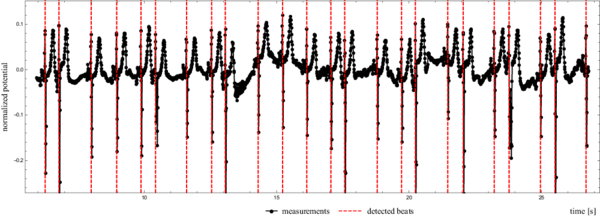
Figure 1 shows how we detected beat to beat times from an actual heartbeat.
A slightly abridged version of the paper is presented below.
Contents
Detection of heart rate variability
from a wearable differential ECG device
Jure Slak, Gregor Kosec, Jožef Stefan Insitute, Department of Communication Systems, Ljubljana.
Abstract
The precise heart rate variability is extracted from an ECG signal measured by a wearable sensor that constantly records the heart activity of an active subject for several days. Due to the limited resources of the wearable ECG device the signal can only be sampled at relatively low, approximately $100$ Hz, frequency. Besides low sampling rate the signal from a wearable sensor is also burdened with much more noise than the standard $12$-channel ambulatory ECG, mostly due to the design of the device, i.e. the electrodes are positioned relatively close to each other, and the fact that the subject is active during the measurements. To extract heart rate variability with $1$ ms precision, i.e. $10$ times more accurate than the sample rate of the measured signal, a two-step algorithm is proposed. In first step an approximate global search is performed, roughly determining the point of interest, followed by a local search based on the Moving Least Squares approximation to refine the result. The methodology is evaluated in terms of accuracy, noise sensitivity, and computational complexity. All tests are performed on simulated as well as measured data. It is demonstrated that the proposed algorithm provides accurate results at a low computational cost and it is robust enough for practical application.
Introduction
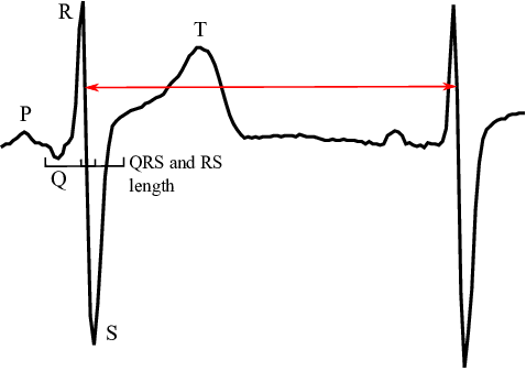
It is well known that the morphology of ECG signals changes from beat to beat as a consequence of physical activity, sensations, emotions, breathing, etc. of the subject. The most straightforward measure of these changes is the heart rate variability (HRV), i.e. small variations of beat duration. HRV characterizes the timings of hearth cells repolarization and depolarization processes. The HRV is typically determined by measuring the intervals between two consecutive R-waves (RRI) or intervals between R and T waves (RTI). Several vital signals can be identified from the HRV and therefore it is often used as a health status indicator in different fields of medicine, e.g. neurology, cardiac surgery, heart transplantation and many more. Typical HRV values of healthy subjects are approximately $40$ ms for RRI and $2$ ms for RTI (see Figure 2). Therefore it is important to detect considered waves with at least $1$ ms accuracy for practical use. This paper deals with the detection of HRV in ECG signal provided by a Wearable ECG Device (WECGD) that is paired with a personal digital assistant (PDA) via Bluetooth Smart protocol. The WECGD, due to the hardware limitations, only measures the signal, while the PDA takes care of data visualization, basic analysis and transmission of the data to a more powerful server for further analyses. In contrast to a standard ambulatory $12$-channel ECG measurement, where trained personnel prepare and supervise the measurement of subject at rest, the WECGD works on a single channel, the subject is active and since the WECGD is often placed by an untrained user its orientation might be random, resulting in additional decrease of signal quality. In order to maintain several days of battery autonomy The WECGD also records the heart rate with significantly lower frequencies and resolution in comparison to ambulatory measurements. All these factors render the standard ECG analysis algorithms ineffective. In this paper we analyse a possible local, i.e. only short history of measurement data is required, algorithm for detection of heart rate variability with $1$ ms precision of a signal recorded with $120$ Hz.
Detection method
In order to evaluate the HRV, the characteristic point of each heart beat has to be detected in the signal, which is provided as values of electric potential sampled with a frequency $120$ Hz. Since the HRV is computed from differences of consequent characteristic points the choice of the characteristic point does not play any role, as long as it is the same in every beat. In this work we choose to characterise the beat with a minimal first derivative, in another words, we seek the points in the signal with the most violent drop in electric potential (Figure 2) that occurs between R and S peaks.
The detection method is separated in two stages, namely global and local. The goal of the global method is to approximately detect the characteristic point, while the local method serves as a fine precision detection, enabling us to detect HRV with much higher accuracy.
Coarse global search
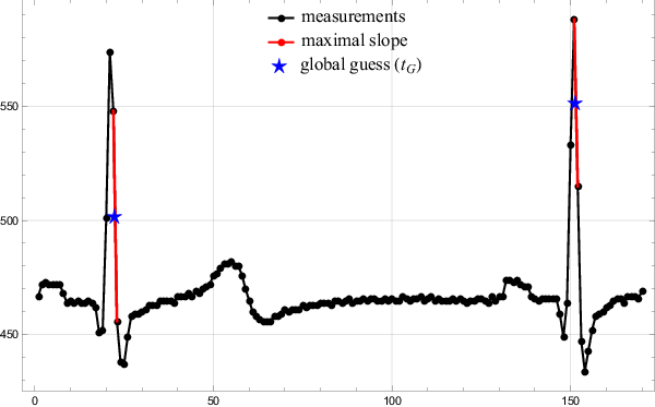
In the first step the algorithm finds a minimal first derivative of a given signal on a sample rate accuracy, i.e. $\frac{1}{\nu}$. The global search method is next to trivial. The algorithm simply travels along the signal, calculating the discrete derivative and storing the position of minimal values found so far. Since the points are sampled equidistantly, minimizing $\frac{\Delta y}{\Delta t}$ is equal to minimizing $\Delta y$. The middle of the interval where the largest drop was detected is taken as the global guess $t_G$. The results of the global search are presented in Figure 3.
Fine local search
The global search provides only coarse, limited to sample points, positions of the characteristic points. To push accuracy beyond $1/\nu$, the signal has to be represented also in between the sample points. A monomial approximation function based on a Moving Least Squares approach is introduced for that purpose.
The value of the electrical potential at arbitrary time $t_0$ is approximated. Denote the vector of $n$ known values near $t_0$ by $\boldsymbol{f}$ (called support), and the times at which they were measured by $\boldsymbol{t}$. The approximation $\hat{f}$ of $\boldsymbol{f}$ is introduced as a linear combination of $m$ in general arbitrary basis functions $(b_j)_{j=1}^m$, however in this work only monomials are considered. \[\hat{f} = \sum_{j=1}^m\alpha_jb_j \]
The most widely used approach to solve above problem and find the appropriate $\hat{f}$ is to minimize the weighted 2-norm of the error, also known as the Weighted Least Squares (WLS) method. \[ \|\boldsymbol{f} - \hat{f}(\boldsymbol{t})\|_w^2 = \sum_{i=1}^n (f_i -\hat{f}(t_i))^2 w(t_i), \] In the above equation $w$ is a nonnegative weight function.
The only unknown quantities are the $m$ coefficients $\boldsymbol{\alpha}$ of the linear combination, which can be expressed as a solution of an overdetermined linear system $W\!B\boldsymbol{\alpha} = W\!\boldsymbol{f}$, where $W$ is the $n\times n$ diagonal weight matrix, $W_{ii} = \sqrt{w(t_i)}$ and $B$ is the $n\times m$ collocation matrix, $B_{ij} = b_j(t_i)$. There are different approaches towards finding the solution. The fastest and also the least stable and accurate is to solve the Normal System $B^\mathsf{T} W^\mathsf{T} WB\boldsymbol{\alpha} = B^\mathsf{T} W^\mathsf{T} W\boldsymbol{f}$, a more expensive but also more stable is via QR decomposition, and finally the most expensive and also the most stable is via SVD decomposition. The resulting vector $\boldsymbol{\alpha}$ is then used to calculate $\hat{f}(t)$ for any given $t$. The derivatives are approximated simply by differentiating the approximating function, $\hat{f}' = \sum_{j=1}^m\alpha_jb_j'$.
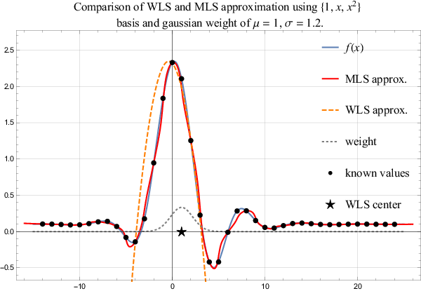
The WLS approximation weights the influence of support points using the weight function $w$. Usually, such a weight is chosen that points closest to $t_0$ are more important in the norm in comparison to the nodes far away. Naturally such approximation is valid only as long as the evaluation point is close to the $t_0$. A more general approach is a Moving Least Square (MLS) approximation, where coefficients $\alpha$ are not spatially independent any more, but are recomputed for each evaluation point. Naturally, such an approach is way more expensive, but also more precise. A comparison of both methods, i.e. WLS and MLS, is shown in Figure 4.
The task of finding the minimal value of the first derivative is equivalent to the task of finding the zero of the second derivative. This zero will be our local approximation $t_L$ of the beat time, $\hat{f}''(t_L) = 0$. Therefore an approximation function with a non constant second derivative, i.e. approximation function with a minimal 3rd order monomial basis, is constructed. The most straightforward approach to find its root is the simple bisection. Bisection requires initial low and high bounds that can be estimated from characteristic point $t_G$ provided by the global method. Using the fact that the QRS intervals last approximately $\Delta t_{\text{QRS}}= 0.1 s$, we can seek for the root of the second derivative on an interval $[t_G - \Delta t_{\text{QRS}}/2, t_G + \Delta t_{\text{QRS}}/2]$, and at given sample rate this translates to the search interval of two sample points away from $t_G$ in each direction.
HRV calculation and error estimation
Given sampled heartbeat, the fine local search produces the vector of $\ell+1$ detected times $\boldsymbol{t_L} := (t_{L,i})_{i=1}^{\ell+1}$ of the RS slopes. Their successive differences represent a vector $\boldsymbol{\hat{r}}$ of detected beat to beat times, the durations of RR intervals. \[ \boldsymbol{\hat{r}} = (\hat{r}_{i})_{i=1}^\ell, \quad \hat{r}_i = t_{L,i+1} - t_{L,i} \] Let $\boldsymbol{r}$ be the vector of (usually unknown) actual beat to beat times. Then the heart rate variability (HRV) $h$ is defined as \[ h := \text{std}(\boldsymbol{r}) = \sqrt{\frac{1}{\ell}\sum_{i=1}^{\ell} (r_i - \bar{r})^2}, \] where $\bar{r}$ stands for the average beat to beat time, $\bar{r} = \sum_{i=1}^\ell r_i / \ell$. The HRV estimation $\hat{h}$ is calculated as the standard deviation of the detected times $\boldsymbol{\hat{r}}$.
In the following analyses the actual vector $\boldsymbol{r}$ will be known, since the synthesized heartbeat will be analysed. The most obvious error measures are the absolute error of HRV, $e_{h} = |\hat{h} - h|$ and the absolute error of the average heart beat $e_{\bar{r}} = |\bar{\hat{r}} - \bar{r}|$. Using the vector of errors $\boldsymbol{e} = |\boldsymbol{r} -\boldsymbol{\hat{r}}|$ the average error $e_a = \sum e_i / \ell$ and the maximal error $e_M = \max(\boldsymbol{e})$ can be assessed.
Results and discussion
Approximation set-up
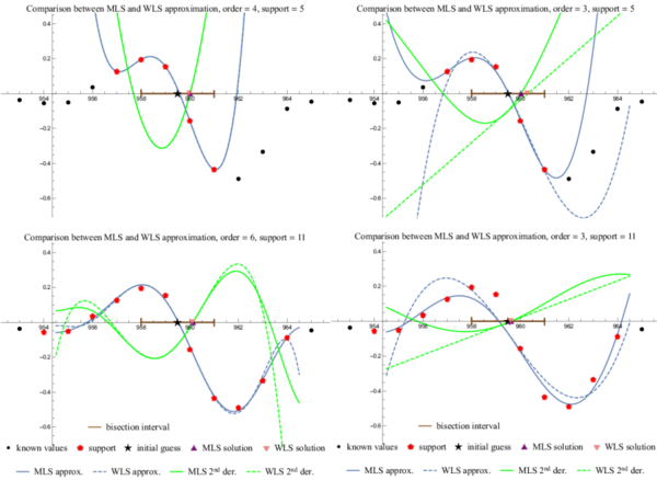
Subfigure a. Sufficiently small support implies interpolation, making weight function useless and MLS equal to WLS.
Subfigure b. MLS and WLS differ when approximating with a low order polynomial.
Subfigure c. MLS and WLS match when approximating with a high order polynomial.
Sunfigure d. Expected bad behaviour with too many support points and a low order approximation.
In first step the approximation free parameters, i.e. weight function, support size, and number of basis functions, have to be assessed. A single heartbeat is extracted and approximated with all possible combinations of basis functions with orders from $2$ to $10$ and symmetric supports of sizes from $3$ to $15$ using both WLS and MLS. An global algorithm described in previous section was used to produce the initial guesses. For demonstration four sample cases are presented. The weight function was the same in all four cases, a Gaussian distribution with $\mu = t_G$ and $\sigma = m/4$, which makes sure that all support points are taken into account, but the central ones are more important.
The simplest case is when the support size is the same as number of basis functions resulting in an interpolation. In this case, the weight function is not important, making WLS and MLS entirely equivalent as seen in Figure 5a.
In case of small support and small order of monomial basis WLS performs worse than MLS and the approaches differ significantly. However, as we increase the order of the polynomial basis the difference within the bisection interval becomes negligible. This transition can be observed in Figure 5b and Figure 5c.
As predicted, the support size is important. Both methods perform badly when too many surrounding measurements are taken into account while still using a low order polynomial approximation. Note that in Figure 5d the initial guess is barely improved and the beat shape is skewed away from the RS drop.
The conclusion is, that for our purposes MLS approximation is unnecessary, as WLS provides good enough results, when used appropriately. Further analysis to determine the best choice of parameters $m$ and $n$ is presented later.
Computational complexity
The presented algorithm is a streaming algorithm, requiring a buffer to store the current beat in the signal. Let $b$ be the number of measurements per beat, stored in a buffer of length $b$. The global part of the algorithm makes $O(b)$ operations, being a simple local search. The local part is more expensive. First a $n \times m$ matrix is constructed in $O(mn)$ and the right hand side vector is copied from the buffer. The system is then solved using SVD decomposition in $O(mn^2+n^3)$ . Note that as $m = O(n)$, this step takes $O(n^3)$. The minimal first derivative is found using bisection. To achieve tolerance $\varepsilon$, $\lceil\log_2(1/\varepsilon)\rceil$ function evaluations are needed, each costing $O(m)$ operations. Total time complexity is therefore equal to $O(b + n^3 + m\log(1/\varepsilon))$. Note, that using MLS would require $O(n^3)$ for each function evaluation, resulting in a significantly worse time complexity of $O(b+n^3\log_2(1/\varepsilon)))$. The calculation of average and variance is done later, after the wanted amount of signal has already been analysed.
In practice the algorithm executes very fast, using typical values $b =
150$, $m=6$, $n=11$ and $\varepsilon = 10^{-10}$ it runs
approximately $0.27$ s to analyze $1000$ heartbeats ($\approx 10^5$ data
points). The algorithm was compiled from C++ source code using
g++5.3.0 with -O2 flag and run on
an Intel(R) Core(TM) i7-4700MQ processor.
Simulated heartbeat with known variability
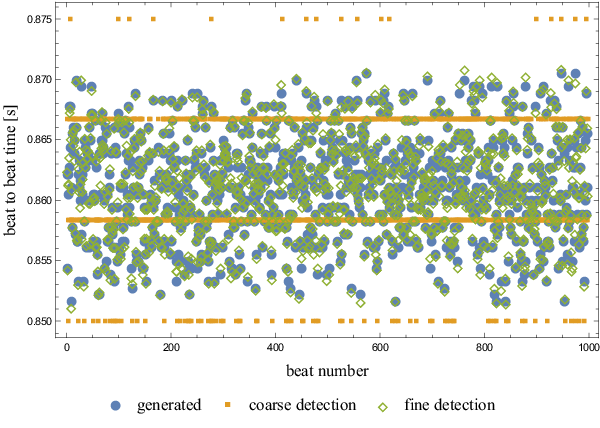
The first set of tests for the presented method was performed using a simulated heartbeat. A single real heartbeat was taken and then replicated thousand times, each time shifted by a random offset $T$, distributed normally around zero, $T \sim \mathcal{N}(0, \sigma^2)$, with $\sigma = \frac{1}{2\nu} = \frac{1}{2} \Delta t$. This means that a decent amount of measurements will be more than $\Delta t$ apart, a difference that must be detected by global search for method to work. However, around half of the measurements are less than $\Delta t$ apart, forming suitable ground for testing the precision of the local search. At given sample frequency, $\sigma$ equals $4.167 ms$.
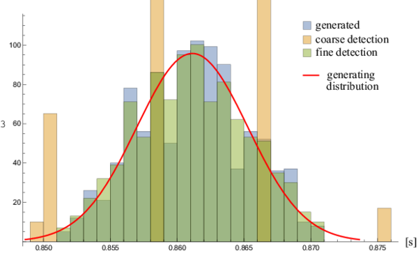
The generated beat to beat times, coarsely detected and finely detected times are presented in Figure 6.
Beat to beat time precision is significantly improved by the local search. As seen in Figure 7, the distributions of generated and detected heart beats match very well.
Results of RRI and HRV detection by global and local search are presented in Table 1. The generated times were taken as precise and the algorithm was run to produce global and local approximations. Then the average RRI time and HRV were calculated for each data set separately. The average RRI time is estimated very well with both methods, but the precision of the global method is not satisfactory when measuring heart rate variability. The precision is significantly improved using the local search. A chart showing the average error of the detected times is shown in Figure 8. It can be seen that MLS performs better on average, but WLS is very close and this loss of precision is a reasonable tradeoff.
The red values in Figure 8 indicate invalid region, having more basis functions than support points. Both MLS and WLS have the same region of validity, being precise in the predicted regime. For very high order approximation the condition number of the matrix becomes critical and the method is unstable, which explains the loss of precision for orders larger than $12$.
| quantity [s] | generated | coarse | fine |
|---|---|---|---|
| $\bar{r} $ | $0.861136$ | $0.861139$ | $0.861136$ |
| $e_{\bar{r}}$ | $0$ | $3.34 \cdot 10^{-6}$ | $2.83 \cdot 10^{-8}$ |
| $h$ | $0.004102$ | $0.005324$ | $0.004137$ |
| $e_h $ | $0$ | $0.001222$ | $3.52 \cdot 10^{-5}$ |
| $e_a $ | $0$ | $0.002969$ | $0.000263$ |
| $e_M $ | $0$ | $0.007778$ | $0.000829$ |
Noise analysis
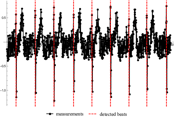
The method presented in this paper relies heavily on the values of the derivative. Normally, derivatives are very sensitive to noise. To analyse noise sensitivity of the algorithm a real heart beat signal was taken and normalized by subtracting the average and then divided by maximal absolute value, transforming measurements onto the interval $[-1, 1]$. A uniform noise of level $p$ was then applied to every measurement. Specifically, a uniformly distributed random number on the interval $[-p, p]$, for fixed $p\in[0, 1]$ was added to every measurement point.
Example of the noised and normalized beat and the behaviour of the algorithm is shown in Figure 9.
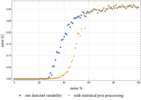
An approximate calculation of the critical noise level can be made. Let $\nu$ be the sample frequency and $p$ the noise level. The critical noise level is such, that the maximal noise derivative is comparable to the maximal derivative of the signal. The maximal noise derivative is achieved when to subsequent measurements take extreme values of $p$ and $-p$, resulting in drop of magnitude $2p$. In the actual heartbeat, the maximal drop appears during R and S peaks. Taking maximal number of nodes in QRS complex to be $\lceil 0.1 \nu \rceil$ as before, and with respect to Figure 1 the RS drop contains at most one third of them, we approximate the maximal drop between two subsequent measurements as the total RS drop divided by number of nodes included. Taking into account that the RS drop equals $2$ after normalization, we obtain \[ \Delta y_{\text{max}} = \frac{2}{\frac{1}{3}\lceil 0.1\nu\rceil} \approx 60 \frac{1}{\nu}. \] The critical noise level is such, that both noise levels are approximately equal \[ 2p_{\text{crit}} \approx 60 \frac{1}{\nu}. \] At sample frequency of $120$ Hz this yields \[ p_{\text{crit}} \approx 0.25. \]
The algorithm was tested as described above for noise levels $p \in [0, 1]$ with a step of $1$%. Results are presented in Figure 10. Note that the rise in error corresponds nicely with predicted critical noise.
A little bit more can be achieved using simple statistical analysis. When noise levels are around critical, a few false beats may be recognized among the actual ones. The RRI time before and after the false beat will deviate greatly from the average RRI time. Therefore, we can choose to ignore extreme values, as they are very likely to be wrong. Average and standard deviation are both sensitive to extreme data points, however the median is not, and while extreme values occur rarely, the median should give a good sense of what the "correct" beat to beat time is. To detect the extreme values a Median Absolute Deviation (MAD) was chosen as the simplest and robust enough approach. In this method, the median of differences from the median is taken as the estimate of data variability. All values that differ more that five times MAD from the median are ignored. The results of applying this technique are also shown in Figure 10.
Actual heartbeat analysis
The presented method was tested on sample inputs from the wearable sensor. Detected beats are presented in Figure 1. Average beat to beat time of the subject was $\bar{\hat{r}} = 0.888264 s$ and heart rate variability equals $\hat{h} = 0.282443 s$.
Conclusion
In this paper a simple MLS based algorithm for accurate detection of HRV from a low sample rate ECG signal, typically provided by a wearable sensor, is demonstrated. The algorithm is formulated in a fairly general way. Most of the approximation parameters can be easily changed. However, to keep the analyses within the reasonable limits, only the order of monomial basis and the support size are varied to find the optimal set-up. It is demonstrated that increasing order of basis as well as support size improves results up to roughly $m=12$ and/or $n=20$, at which point the system matrix becomes ill-conditioned. Based on the presented analyses a basis of $10$th order supported with $15$ nodes is claimed to be the optimal set-up. It is also demonstrated that using a way more computationally expensive MLS, in comparison to WLS, do not improve accuracy enough to justify it.
Based on results from approximation analyses a fast two-stage streaming algorithm for HRV detection is developed. The algorithm is tested on synthetic as well as actual data, achieving good performance. It is demonstrated that the detected beat times of a simulated heartbeat differ from the actual ones with an average absolute error of $0.263$ ms at sample frequency of $120$ Hz. In other words the detection accuracy is roughly ten times more accurate in comparison with a coarse one. The method is also stable up to approximately $25$% noise and computationally extremely effective, successfully processing $1000$ heartbeats in approximately $0.27$ s on a standard laptop computer.
In future work we will focus on full analysis, including different basis and weight functions, as well as non-linear MLS to fit also the basis shape parameters.
