Integrators for time stepping
This page describes how to solve ordinary differential equations numerically with examples from our library.
Contents
Introduction and notation
We are solving an initial value problem, given as
$ \begin{align*} \dot{y}(t) &= f(t, y) \\ y(t_0) &= y_0 \end{align*} $
where $y$ is the unknown (possibly vector) function, $t_0$ is the start time, $f$ is the derivative (the functions we wish to integrate) and $y_0$ is the initial value of $y$. Numerically, we usually choose a time step $\Delta t$ and integrate the function up to a certain time $t_{\max}$. Times of subsequent time steps are denoted with $t_i$ and function values with $y_i$.
The simplest method is explicit Euler's method: $y_{n+1} = y_{n} + \Delta t f(t, y_n)$
Explicit (single step) methods
A family of single step methods are explicit Runge-Kutta methods, which use intermediate derivative values to give a better estimation of value $y_{n+1}$ on the next step.
It is given by
$y_{n+1} = y_n + h \displaystyle \sum_{i=1}^s \beta_i k_i$
where
$ \begin{align*} k_1 & = f(t_n, y_n), \\ k_2 & = f(t_n+\gamma_2h, y_n+h(\alpha_{21}k_1)), \\ k_3 & = f(t_n+\gamma_3h, y_n+h(\alpha_{31}k_1+\alpha_{32}k_2)), \\ & \ \ \vdots \\ k_s & = f(t_n+\gamma_sh, y_n+h(\alpha_{s1}k_1+\alpha_{s2}k_2+\cdots+\alpha_{s,s-1}k_{s-1})). \end{align*} $
To specify a particular method, one needs to provide the integer $s$ (the number of stages), and the coefficients $\alpha_{ij}$, $\beta_i$ and $\gamma_i$. This structure is known as the Butcher's tableau of the method: $ \begin{array}{l|l} \gamma & \alpha \\ \hline & \beta^\T \end{array} $
First order method is the Euler's method above, while methods of very high order are available. The most famous is RK4, the Runge Kutta method of fourth order.
$\begin{align*} & {{k}_{1}}=f({{t}_{i}},{{y}_{i}}) \\ & {{k}_{2}}=f({{t}_{i}}+\Delta t/2,{{y}_{i}}+\Delta t{{k}_{1}}/2) \\ & {{k}_{3}}=f({{t}_{i}}+\Delta t/2,{{y}_{i}}+\Delta t{{k}_{2}}/2) \\ & {{k}_{4}}=f({{t}_{i}}+\Delta t,{{y}_{i}}+\Delta t{{k}_{3}}) \\ & {{y}_{i+1}}={{y}_{i}}+\Delta t/6({{k}_{1}}+2{{k}_{2}}+2{{k}_{3}}+{{k}_{4}}). \\ \end{align*}$
A more complete list can be found here.
Most common methods are implemented in the Explicit namespace.
Explicit multistep methods
These methods are called Adams–Bashforth methods, and need previous $s$ are used to estimate next value with a higher order. These method hope to gain computational efficiency by decreasing the number of function computations needed by using already computed values.
The explicit version is stated as $y_{n+s} = y_{n+s-1} + \sum_{i=1}^s b_i y_{n+s-i}$. The values $b_i$ are called weights.
The drawbacks of these mehtods are that another method of same order is needed to compute the initial time steps and that they can not be easily modified to work with adaptive time steps.
Most common methods are implemented in ExplicitMultistep namespace.
Adaptive methods
Adaptive methods estimate the error on each time step and descrease or increase the step as necessary. Usually the have some addition parameters, such as $\Delta t_{\max}$ and $\Delta t_{\min}$ representing maximal and minimal allowed time steps and $\varepsilon$, represeting tolrance.
A family of adaptive methods can be derived from Runge Kutta methods above. Using a method of order $k$ and $k+1$, that differ only in weights, called $\beta$ and $\beta^\ast$, error can be estimated using Richardson Extrapolation:
$e_{n+1} = y_{n+1} - y^*_{n+1} = h\sum_{i=1}^s (\beta_i - \beta^*_i) k_i$.
If $\|e_{n+1}\| < \varepsilon$, time step can be increased, otherwise it is decreased. This can be achieved by scaling $\Delta t$ in accorance with $\varepsilon / \|e_{n+1}\|$.
These methods are implemented in Matlab as ode45 and similar. They can be found here, with a sample Matlab implementation of Cash-Karp method here.
These methods are not implemented yet, but will probably be added in the future.
Usage
Ordinary ODE: Solve $\dot{x} = y, \dot{y} = -x$ with $x(0) = 1, y(0) = 0$.
// define the function
std::function<Eigen::VectorXd(double, const Eigen::VectorXd&)> func =
        [](double, const Eigen::VectorXd& y) {
            Eigen::VectorXd r(2);
            r(0) = -y(1);
            r(1) = y(0);
            return r;
        };

double tmax = 2*M_PI;
double step = 0.1;
Eigen::VectorXd y0(2); y0 << 1.0, 0.0;
auto integrator = integrators::Explicit::RK4().solve(func, 0.0, tmax, step, y0);  // clss representing the method and storing the function and initial conditions.

auto stepper = integrator_rk4.begin();  // iterator over the solver, integrating $f$ step by step

while (stepper_rk4) {  // cast to bool tells us if we are done
    ++stepper_rk4;
    // do something with step
}

// multiple steppers can exists at the same time
auto stepper2 = integrator.begin();

// we can also use range based for loop to integrate by time
for (auto& step : integrator) {
   //  do something with step
}
Heat equation:
// after domain and operators are created
auto dv_dt = [&](double, const VecXd& y) {
    Eigen::VectorXd der(y.size());
    for (int c : interior) {
        der[c] = op.lap(y, c);
    }
    for (int c : boundary) {
        der[c] = 0;
    }
    return der;
};

auto integrator = integrators::Explicit::RK4().solve(dv_dt, 0.0, time, dt, T1);  // choose your own integrator
for (auto& step : integrator) {
   // do something
}
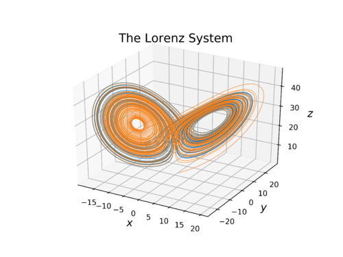
// System parameters
double sigma = 10.;
double rho = 28.;
double beta = 8./3.;

auto dy_dt = [&](double, const Vec3d& y) {
    Vec3d der(3);
    der(0) = sigma*(y(1)-y(0));
    der(1) = y(0)*(rho-y(2))-y(1);
    der(2) = y(0)*y(1)-beta*y(2);
    return der;
};

double dt = 0.001; // Timestep
Vec3d y0 = {1, 1, 1}; // Initial condition

auto integrator = integrators::Explicit::RK4().solve(dy_dt, 0, 100, dt, y0);
for (auto& step : integrator) {
    auto t = step.time();
    auto y = step.value();
    // output values
}
