Coupled domains
Go back to Examples.
In this example we will show how one can solve coupled problems with the Medusa library. We will solve the stationary heat equation on concentric circles where the thermal conductivity $\lambda$ is different for each circle. The inner circle will be heated up, while the outside temperature will be held at zero.

In mathematical terms, we want to solve the following system for two unknown function $u$ and $v$ \begin{align*} -\lambda_2\Delta v = q_0 \qquad &\text{on} \quad \Omega_2 \\ \lambda_1\Delta u = 0 \qquad &\text{on} \quad \Omega_1 \end{align*} with boundary conditions \begin{align*} u = 0 \qquad &\text{on} \quad \partial \Omega_1 \\ u = v \qquad &\text{on} \quad \partial \Omega_2 \\ \lambda_2 \frac{\partial u}{\partial n} + \lambda_1 \frac{\partial v}{\partial n} = 0 \qquad &\text{on} \quad \partial \Omega_2. \\ \end{align*} We will see that the task is quite simple using Medusa.
Discretisation
First we create the domains $\Omega_1$ and $\Omega_2$
 1     BallShape<Vec2d> inner_shape(0, r1);
 2     BallShape<Vec2d> outer_circle(0, r2);
 3     auto outer_shape = outer_circle - inner_shape;
 4
 5     DomainDiscretization<Vec2d> outer = outer_shape.discretizeBoundaryWithStep(h);
 6     DomainDiscretization<Vec2d> inner(inner_shape);
 7
 8     // Indices of nodes in outer domain that constitute outer and common boundary.
 9     auto common_bnd = outer.positions().filter([=](const Vec2d& p) { return std::abs(p.norm() - r1) < 1e-5; });
10     auto outer_bnd = outer.positions().filter([=](const Vec2d& p) { return std::abs(p.norm() - r2) < 1e-5; });
In the code above, we constructed two BallShapes and calculated their difference, giving us the shape of an annulus. We use the annulus shape to obtain the outer domain discretization, and the BallShape with the smaller radius to construct the inner domain discretization. Some care needs to be given to filling the domains, because we want the domains to have the same node coordinates on the common boundary $\partial \Omega_2$. Note that as we discretized the boundary of the annulus we already filled both $\partial \Omega_1$ and $\partial \Omega_2$. Hence, we split the boundary nodes of the outer domain into the outer boundary and the common boundary, which will prove useful later on.
 1     // Maps node indices of outer domain to their corresponding indices in the inner domain.
 2     Range<int> outer_to_inner(outer.size(), -1);
 3     for (int i : common_bnd) {
 4         int idx = inner.addBoundaryNode(outer.pos(i), -2, -outer.normal(i));
 5         outer_to_inner[i] = idx;
 6     }
 7
 8     GeneralFill<Vec2d> fill_engine; fill_engine.seed(1);
 9     outer.fill(fill_engine, h); // this is the annulus
10     inner.fill(fill_engine, h); // this is the inner circle
The snippet above shows how to add the the nodes on the common boundary to the inner domain. The normals of the shared boundary nodes belonging to the inner domain must point into the opposite direction as the normals belonging to the shared boundary nodes in the outer domain. Additionally, mapping of node indices from outer domain to the index of the same node in the inner domain was made. After this is done, the insides of both domains are filled.
Assembling and solving the system
The size of the matrix $M$ of the system must be equal to the sum of numbers of nodes in the inner and outer domains.
1     Eigen::SparseMatrix<double, Eigen::RowMajor> M(N_inner+N_outer, N_inner+N_outer);
2     Eigen::VectorXd rhs(N_inner+N_outer);
Additionaly we must construct two sets of storages, and two sets of operators, one for each domain. The operators of the outer domain must be offset by the number of nodes in the inner domain. This assures that the operators are writing values in the correct part of the matrix $M$.
1     auto storage_inner = inner.computeShapes<sh::lap|sh::d1>(wls);
2     auto storage_outer = outer.computeShapes<sh::lap|sh::d1>(wls);
3
4     auto op_inner = storage_inner.implicitOperators(M, rhs);
5     auto op_outer = storage_outer.implicitOperators(M, rhs);
6     op_outer.setRowOffset(N_inner);
7     op_outer.setColOffset(N_inner);
On the shared boundary we must reserve two slots for the equality of values of $u$ and $v$, and the appropriate number of slots to store two shapes due to equality normal derivatives of $u$ and $v$.
1     Range<int> reserve = storage_inner.supportSizes() + storage_outer.supportSizes();
2     // Compute row sizes on the common boundary
3     for (int i : common_bnd) {
4         reserve[outer_to_inner[i]] = 2;  // equality of values needs 2 slots
5         reserve[N_inner+i] = storage_inner.supportSize(outer_to_inner[i]) + storage_outer.supportSize(i);  // equality of fluxes needs two shapes
6     }
7     M.reserve(reserve);
Finally we can implement the case, being careful to write in the appropriate parts of the matrix when dealing with shared points. When we filtered the indexes into the common_bnd vector we used the indexes of the nodes in the outer domain, we use the mapping outer_to_inner to obtain the indexes corresponding to the same nodes in the inner domain.
 1     for (int i : inner.interior()) {
 2         -lam1*op_inner.lap(i) = q0;  // laplace in interior of inner domain
 3     }
 4     for (int i : outer.interior()) {
 5         lam2*op_outer.lap(i) = 0;  // laplace in interior of outer domain
 6     }
 7     for (int i : outer_bnd) {
 8         op_outer.value(i) = 0.0;  // outer Dirichlet BC
 9     }
10     for (int i : common_bnd) {
11         int j = outer_to_inner[i];
12         op_inner.value(j) + -1.0*op_outer.value(i, -N_inner+j) = 0.0; // continuity over shared boundary
13         lam1*op_inner.neumann(j, inner.normal(j), N_inner+i) + lam2*op_outer.neumann(i, outer.normal(i)) = 0.0; // flux continuity
14     }
The annotated sparse matrix representing the coupled system is shown below.

The only thing that remains to be done is to solve the system of equations we obtained. Depending on the relative values of $\lambda_1$ and $\lambda_2$ we may obtain two types of solutions
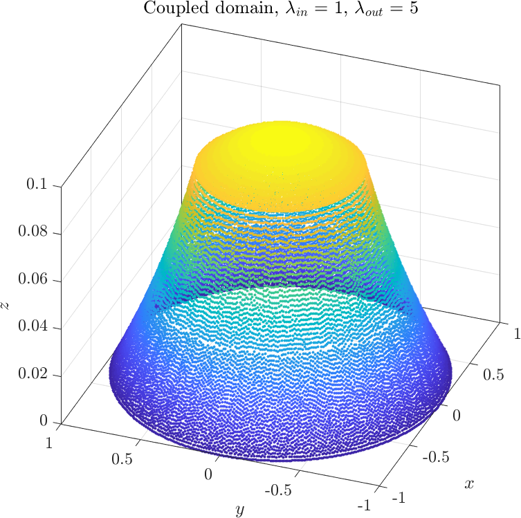
We obtain a "volcano" shape if $\lambda_1 < \lambda_2$
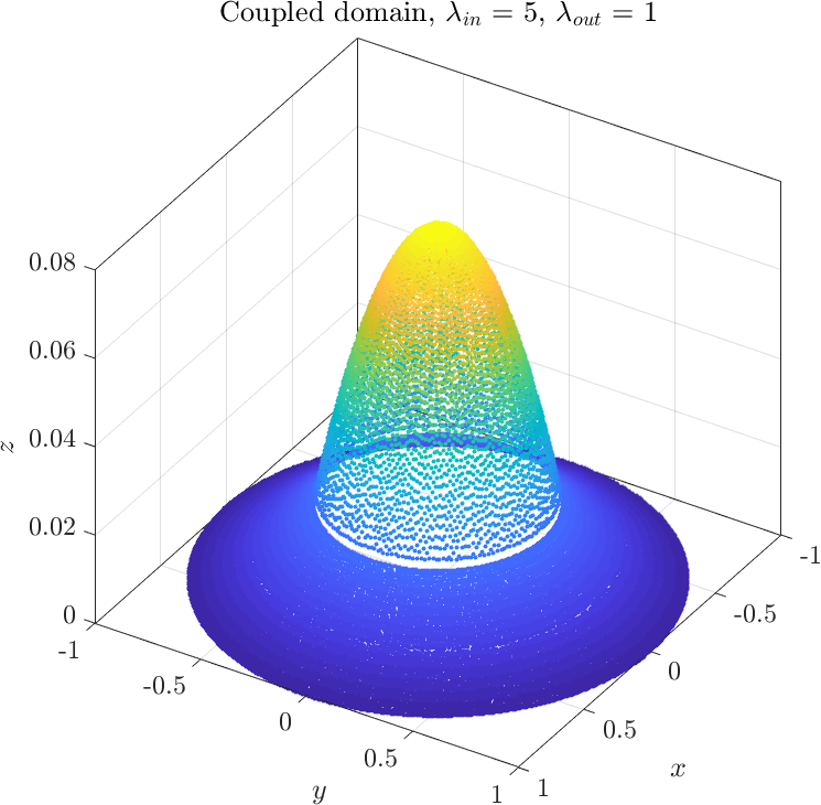
We obtain a "sombrero" shape if $\lambda_1 > \lambda_2$


The example can be found here poisson_coupled_domains.cpp, and the matlab plot script as poisson_coupled_domains.m.
Go back to Examples.