Cahn-Hilliard equation
Go back to Examples.
In this example we will show how to solve the Cahn-Hilliard equation in Medusa. The solution provides an implementation of periodic boundary conditions and shows how to combine implicit and explicit operators. This example uses a custom biharmonic operator, so we recommend firstly reading the tutorial on Customization.
Contents
Cahn-Hilliard equation
The Cahn-Hilliard equation describes the separation of binary fluid into pure domains. We define concentration, a scalar field $c(x, y) \in [-1, 1]$ to describe the fluid, with values $c \pm 1$ representing pure phases. In this case the equation can be written as
\[ \frac{\partial c}{\partial t} = D \nabla^2 (c^3 - c - \gamma \nabla^2 c), \] where $D$ is the diffusion constant and $\sqrt{\gamma}$ is the characteristic transition length between domains.
We want to avoid any boundary effects and solve the equation for infinite fluid which can be approximated by using periodic boundary conditions.
Periodic boundary conditions

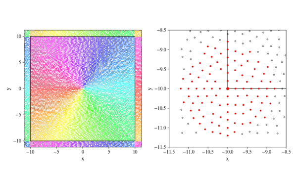
Figure 1: Periodic band display.
Left subplot shows an example of filled domain with $border = 10$ and $dx = 0.2$. Interior nodes and their periodic counterparts share colors to illustrate periodicity.
Right subplot shows the neighbourhood of bottom left corner node $(-border, -border)$, with its support nodes highlighted in red. This example uses same fill parameters as the left figure and a support size of 100.
The simplest method of implementing a periodic boundary is adding a band of periodic nodes that mirror values from nodes that lie close to the opposite boundary. We have to create periodic nodes based on locations of interior nodes and construct a mapping that will allow us to update their values based on their interior counterparts. Width of the periodic band should be chosen with support size in mind. Periodic band should be wide enough to include all nodes required to calculate interior values. An example that can help us determine the required width of the periodic band is shown on the right subplot of Figure 1 and shows that we need a periodic band width of $6 dx$ for a support size of 100.
We start by creating a square domain centered on 0 and uniformly filling it with nodes. $border$ parameter determines the square size while $dx$, the typical distance between nodes, determines the node density.
mm::BoxShape<vec_t> box(-border, border);
mm::DomainDiscretization<vec_t> domain = box.discretizeBoundaryWithStep(dx);
mm::GeneralFill<vec_t> fill;
fill.seed(randomSeed);
domain.fill(fill, dx);
Afterwards we remove boundary nodes at positive $border$ and move others into interior. This creates a $[-border, border) \times [-border, border)$ interior that can be made periodic.
Eigen::Matrix2d borders;  // col1: - border, col2: + border, rows for dimensions
borders << domain.shape().bbox().first, domain.shape().bbox().second;
for (auto idx : domain.boundary()) {
    const auto& pos = domain.pos(idx);
    if (pos[0] != borders(0, 1) && pos[1] != borders(1, 1)) {
        domain.changeToInterior(idx, pos, 1);
    }
}
domain.removeBoundaryNodes();
Now we are ready to find all nodes that lie sufficiently close to the border and create their periodic counterparts. In general rectangle case we would need to check all dimesions and create periodic nodes in all subsets of dimensions where that node lies close to the border. In this 2D case that simplifies to checking whether node lies close to the border in $x$, $y$ or both, which would mean a periodic corner. We could simplify our code and ignore the small periodic corners but that would lead to slightly worse results.
Periodic boundary nodes are created with type -2 so that we can still differentiate between them and any legitimate boundary nodes we would have in case of mixing periodic and normal boundary conditions. Boundary normal can be chosen arbitrarily, periodic nodes are only used as value holders.
During this process we also store periodic node indices in $periodicNodes$ and indices of the original nodes in $interiorMapping$.
mm::Range<int> periodicNodes;
mm::Range<int> interiorMapping;
mm::Vec2d normal(0, 0);  // not used in this case and can be chosen arbitrarily
for (auto idx : domain.interior()) {
    const auto& pos = domain.pos(idx);
    // col1: distance to - border, col2: distance to + border, rows represent dimensions
    auto borderDistance = borders.colwise() - pos;
    const auto& isPeriodic = borderDistance.array().abs() < periodicBandWidth * dx;
    for (int i0 = 0; i0 < 2; i0++) {
        // check for periodicity in 1st dimension (x)
        if (isPeriodic(0, i0)) {
            auto periodicPos = pos;
            periodicPos(0) = borders(0, (i0 + 1) % 2) - borderDistance(0, i0);
            periodicNodes.push_back(domain.addBoundaryNode(periodicPos, -2, normal));
            interiorMapping.push_back(idx);
        }
        for (int i1 = 0; i1 < 2; i1++) {
            // check for periodicity in 2nd dimension (y)
            if (i0 == 0 && isPeriodic(1, i1)) {
                auto periodicPos = pos;
                periodicPos(1) = borders(1, (i1 + 1) % 2) - borderDistance(1, i1);
                periodicNodes.push_back(domain.addBoundaryNode(periodicPos, -2, normal));
                interiorMapping.push_back(idx);
            }
            // check for periodicity in both dimensions (corners)
            if (isPeriodic(0, i0) && isPeriodic(1, i1)) {
                auto periodicPos = pos;
                periodicPos(0) = borders(0, (i0 + 1) % 2) - borderDistance(0, i0);
                periodicPos(1) = borders(1, (i1 + 1) % 2) - borderDistance(1, i1);
                periodicNodes.push_back(domain.addBoundaryNode(periodicPos, -2, normal));
                interiorMapping.push_back(idx);
            }
        }
    }
}
Solution
We need to handle two uncommon terms to solve the equation. Biharmonic ($\nabla^4$) operator can be implemented with custom operators as shown in Customization example. Nonlinear ($\nabla^2 c^3$) term proves to be more problematic, as it can not be solved implicitly. We either need to solve the entire equation with explicit time stepping or include the nonlinear term in the right hand side of our system of equations.
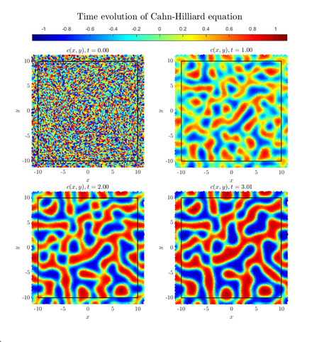
Initial concentration is random.
Explicit solution
Explicit solution is simpler to implement and faster when we want to solve the equation for very small time steps.
We use Euler method for time stepping and copy interior node values to their periodic counterparts at every step.
double t = 0;
Eigen::VectorXd bracket;
while (t <= tEnd) {
    bracket = concentration.array() * concentration.array() * concentration.array() - concentration.array();
    for (int i : allNodes) {
        bracket[i] -= L * expOp.lap(concentration, i);
    }
    for (int i : interiorNodes) {
        concentration[i] = concentration[i] + dt * D * expOp.lap(bracket, i);
    }
    t += dt;

    for (int i = 0; i < periodicSize; i++) {
        concentration[periodicNodes[i]] = concentration[interiorMapping[i]];
    }
}
Mixed solution
Mixed solution allows for much longer (several orders) time steps as we solve the majority of our equation implicitly. Explicit computation of the nonlinear term will always lead to inaccuracies, especially for long $dt$.
We set the equation on interior and identities on boundary.
for (int i : interiorNodes) {
    impOp.value(i) + D * dt * impOp.lap(i) + D * dt * L * impOp.apply<Biharmonic<dim>>(i) = rhs[i];
}
for (int i = 0; i < periodicSize; i++) {
    impOp.value(periodicNodes[i]) = rhs[interiorMapping[i]];
}

Eigen::SparseLU<decltype(M)> solver;
solver.compute(M);
We have to explicitly compute nonlinear $\nabla^2 c^3$ term at every step and add it to the rhs. Once we solve the system for new concentration we have to copy interior node values to their periodic counterparts.
/// Time stepping.
double t = 0;
Eigen::VectorXd cubedConcentration;
while (t <= tEnd) {
    /// Prepare rhs.
    cubedConcentration = concentration.array() * concentration.array() * concentration.array();
    for (int i : allNodes) {
        concentration[i] = D * dt * expOp.lap(cubedConcentration, i) + concentration[i];
    }

    concentration = solver.solve(concentration);
    t += dt;

    /// Copy values from interior nodes to their periodic representations.
    for (int i = 0; i < periodicSize; i++) {
        concentration[periodicNodes[i]] = concentration[interiorMapping[i]];
    }
}
The complete example is avalible on git.
Go back to Examples.
