Non-Newtonian fluid

Click here to return back to Fluid Mechanics

Introduction

Other fluid mechanics examples have assumed that the fluids in question are Newtonian, but that is not always the case when dealing with real world applications. Many significant fluids exhibit non-Newtonian behaviour with examples including blood, foodstuffs, polymer melts... Newtonian fluids have a linear relationship between viscous stress and shear rate but that is no longer true for non-Newtonian fluids.

Some fluids exhibit increasing or decreasing viscosity with increasing shear rate which is the simplest form of non-Newtonian behaviour that we will tackle in the following sections. Some act as solids at small stress but begin flowing when sufficiently disturbed, while others behaviour depends on the duration of movement and applied stress.

Model formulation

Viscous forces are a result of velocity differentials within the fluid and are therefore connected with the velocity gradient. We are interested in the symmetric part that excludes the rotational contributions. Shear rate tensor $\dot{u}$ for incompressible fluids can be expressed as $$ \dot{u}=\frac{1}{2}\left(\boldsymbol{\nabla} \boldsymbol{v}+(\boldsymbol{\nabla} \boldsymbol{v})^{\top}\right), $$ where $\boldsymbol{v}$ denotes the fluid velocity. We introduce viscosity $\mu$ through a generalized Newton's law of viscosity with viscous stress tensor $\tau$ expressed as $$ \tau = \mu \dot{u}. $$ In general $\mu$ is an arbitrary tensor but usually reduces to a scalar value due to isotropic properties of fluids. Non-Newtonian fluids are fluids where viscosity is a function of shear stress and duration of stress. There are many, often quantitative, models of varying complexities used to describe the viscosity of various non-Newtonian fluids.

We limit ourselves to Ostwald-de Waele power law model $$ \mu = \mu_0 \left\| \dot{u} \right\| ^{n-1} = \mu_0 \left( 2 \dot{u}{:}\dot{u} \right) ^\frac{n-1}{2}, $$

Figure 1: Scheme of the de Vahl Davis benchmark test.

which is one of the simplest non-Newtonian viscosity models. We introduced two parameters used to fit the model to the experimental data for the fluid in question. Viscosity constant $\mu_0$ used as a scaling factor and non-Newtonian power index $n$ that describes the behaviour. Model with $n < 1$ describes shear-thinning (pseudoplastic), $n = 1$ Newtonian and $n > 1$ shear thickening (dilatant) fluids.

We will focus on shear thinning fluids as their behaviour of reduced viscosity at higher velocity gradients leads towards interesting behaviour with decreasing $n$.

non-Newtonian de Vahl Davis case

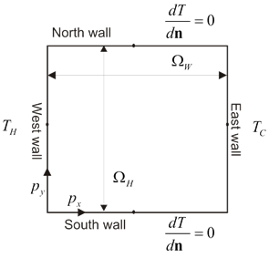
We take a closer look at the behaviour of non-Newtonian fluid in a natural convection driven flow within a square cavity. The convection is driven by differentially heated east and west walls with the north and south walls thermally insulated as is schematically shown in Figure 1.

This example is similar to the explicit pressure correction described in the de Vahl Davis natural convection test with the addition of the non-Newtonian viscosity $\mu$ modeled with the Ostwald-de Waele power law $$ \mu = \mu_0 \left\| \frac{1}{2}\left(\boldsymbol{\nabla} \boldsymbol{v}+(\boldsymbol{\nabla} \boldsymbol{v})^{\top}\right) \right\| ^{n-1}, $$ where $\mu_0$ denotes the viscosity constant, $\boldsymbol{v}$ the fluid velocity and $n$ the non-Newtonian power index. The model parameters $\mu_0$ and $n$ for specific fluids are usually determined from experimental data.

We will solve the natural convection driven problem in a square cavity that is schematically shown in Figure 1. The north and south walls are thermally insulated while the east and west walls are kept at constant but different temperatures. Different temperatures lead to differing fluid densities that cause natural convection. The problem is defined with a system of coupled partial differential equations $$ \begin{aligned} \boldsymbol{\nabla} \cdot \boldsymbol{v} &=0, \\ \rho \frac{\mathrm{D} \boldsymbol{v}}{\mathrm{D} t} &=-\boldsymbol{\nabla} p+\boldsymbol{\nabla} \cdot(\mu \boldsymbol{\nabla} \boldsymbol{v})-\boldsymbol{g} \rho \beta \small{\Delta} T, \\ \rho c_{p} \frac{\mathrm{D} T}{\mathrm{D} t} &=\boldsymbol{\nabla} \cdot(\lambda \boldsymbol{\nabla} T), \end{aligned} $$ where $\rho$ denotes the density, $\boldsymbol{g}$ the gravitational acceleration, $\beta$ the thermal expansion coefficient, $T$ temperature, $c_p$ the specific heat capacity and $\lambda$ the thermal conductivity. Equations are written using the material derivative $$\frac{\mathrm{D x}}{\mathrm{D} t}=\frac{\partial x}{\partial t}+\boldsymbol{v} \cdot \boldsymbol{\nabla} x,$$ that stems from describing the conservation laws for a moving fluid in terms of property values at fixed positions.

Natural convection is implemented by coupling the temperature and velocity equations with Bousinessq approximation. We assume that the thermal variations in density are small and can be neglected where not multiplied by the gravitational acceleration. This assumes that the other acceleration is small, which is true while the weak convective force remains relevant for the dynamics.

Hydrostatics contained in $p$ are irrelevant for this problem and can be omitted to reduce complexity and improve stability.

Majority of the solution process is similar to the explicit pressure correction example referenced above. The solution process diverges in the time step calculation for the velocity field where we have to account for the changing viscosity.

for (i = 0; i < domain.size(); ++i) {
    v_grad[i] = op_v.grad(u_1, i);
    double norm = ((v_grad[i] + v_grad[i].transpose())).squaredNorm() / 2;
    // limit minimal norm value to avoid infinite viscosity
    norm = std::max(norm, EPS);
    viscosity[i] = mu * std::pow(norm, (power_index - 1) / 2);
}

for (i = 0; i < interior.size(); ++i) {
    int c = interior[i];
    u_2[c] = u_1[c] + dt * ((v_grad[c] * op_s.grad(viscosity, c)
                             + viscosity[c] * op_v.lap(u_1, c)) / rho
                             - v_grad[c] * u_1[c]
                             - g * (beta * (T_1[c] - T_ref)));
}

The first loop calculates the field of viscosity values that is needed to calculate the viscosity derivative at the next step. We store the velocity gradient values as they will be reused in the following computations. Non-Newtonian viscosity is calculated from the magnitude of the symmetric part of the velocity gradient defined as $ \dot{u}=\frac{1}{2}\left(\boldsymbol{\nabla} \boldsymbol{v}+(\boldsymbol{\nabla} \boldsymbol{v})^{\top}\right)$ that we calculate using the tensor magnitude formula $\left\| x \right\| = \sqrt{2\,x{:}x}$. The norm values are lower bounded by a small EPS$=10^{-10}$ value to avoid infinite viscosities at small shear rates in shear thinning ($n < 1$) fluids.

The second loop is the actual time step for Euler discretized velocity equation. We separate $\boldsymbol{\nabla} \cdot(\mu \boldsymbol{\nabla} \boldsymbol{v}) = \boldsymbol{\nabla}\mu \boldsymbol{\nabla} \boldsymbol{v} + \mu \nabla^2 \boldsymbol{v}$ to avoid calculating the divergence of a tensor field.

The code is available as nonNewtonian_fluid.cpp in the Medusa examples.

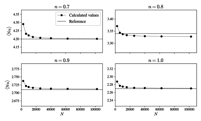
This is a common benchmark with existing solutions that we can compare our meshless implementation against. Convergence and comparison with the benchmark article is shown in Figure 2 where we plot how the average Nusselt number changes with increasing node density. Nusselt number is a dimensionless number that expresses the ratio between the convective and conductive heat transfer. We use the average value on the western wall and define it as

Figure 2: Convergence of the average Nusselt number value with the increasing node count and comparison with reference values from the reference. Convergence is calculated at Ra$=10^4$ and Pr$=10$.

$$ \mathrm{Nu}=\frac{\Omega_W}{T_{H}-T_{C}}\left|\frac{\partial T}{\partial p_x}\right|_{p_x=0}, $$ where $T$ denotes the temperature, $p_x$ the $x$ coordinate and $\Omega_W$ the cavity width. Nusselt number is a convenient tool that can be used to reduce the dynamics of a complex multidimensional system into a single scalar value.

We define the problem in terms of Rayleigh and Prandtl dimensionless numbers that need to be slightly modified to remain relevant in a non-Newtonian case but their specifics are not really relevant for this review. Dimensionless number definitions used in these calculations match reference and can be viewed there.

Parameters that lead to an oscillatory behaviour in the de Vahl Davis cavity can be found in literature. The referenced article found oscillatory behaviour in Newtonian fluids at Ra=$5 \cdot 10^4$ and Pr=$0.01$, but we want to use a slightly lower Ra value to find the transition as the dynamics become wilder with a smaller $n$. We chose Ra=$2 \cdot 10^4$ and Pr=$0.01$ as the parameters to be used for all subsequently displayed calculations.

The following figures display or mention dimensionless time that is defined with the same definition as described in the reference.

Figure 3: Evolution of the average Nusselt number in a differentially heated square cavity for different values of the non-Newtonian power index $n$.

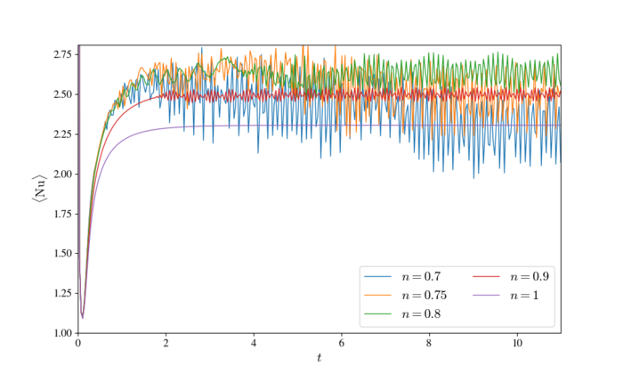
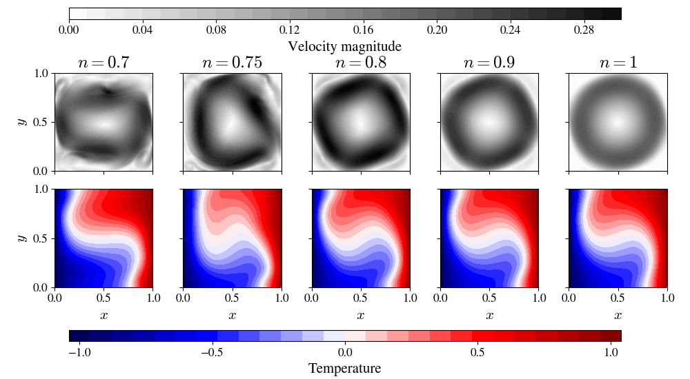
We reuse the Nusselt number to analyse the differences in behaviour for different non-Newtonian power indices $n$ shown in Figure 3. The Newtonian case with $n=1$ settles into a stationary case which is expected, as we chose parameters below the previously identified oscillatory solution. The time evolutions of the average Nusselt number become oscillatory as we increase the strenght of non-Newtonian behaviour, while the solutions become less and less regular as we reduce the power index $n$, which can be seen in pictures of velocity and temperature distributions shown in Figure 4. Detailed animation of behaviour in the most extreme $n=0.7$ case is shown in Figure 5.

Exact implementation of the non-Newtonian fluid modeled with Ostwald-de Waele power law can be found in the example.

Figure 4: Velocity and temperature fields within the cavity at $t=10$ for different values of the non-Newtonian power index $n$.

Figure 5: Animation of velocity and temperature fields within the cavity between $t=10$ and $t=11$ for $n=0.7$.

Go back to Examples.

References

- ↑ 1.0 1.1 O. Turan, A. Sachdeva, N. Chakraborty in R. J. Poole, Laminar natural convection of power-law Fluids in a square enclosure with differentially heated side walls subjected to constant temperatures, Journal of Non-Newtonian Fluid Mechanics 166, 1049 (2011).
- ↑ 2.0 2.1 G. Kosec in B. Šarler, Solution of a low Prandtl number natural convection benchmark by a local meshless method, International Journal of Numerical Methods for Heat & Fluid Flow 23, 22 (2013).