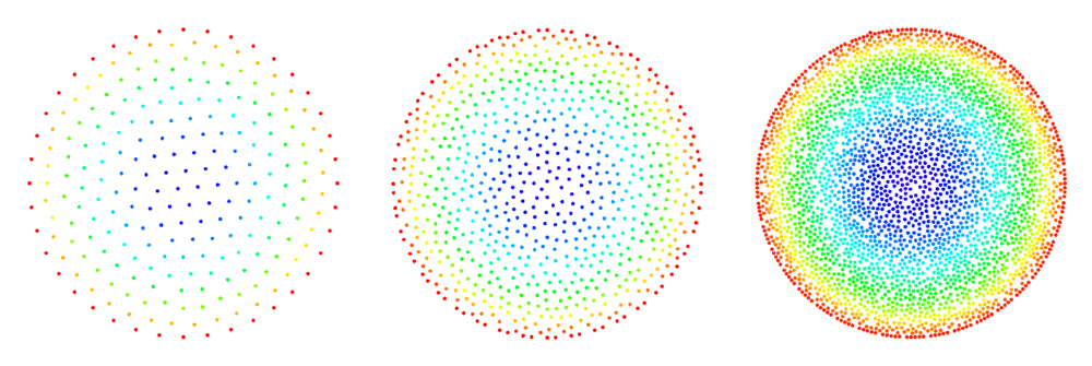
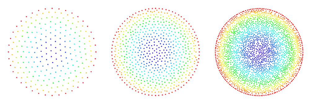
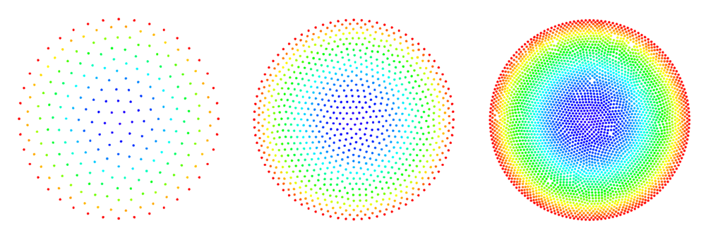
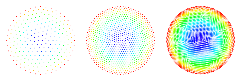
Positioning of computational nodes

Since one of the most attractive features of mesh-free methods is the ability to use nodes without any connectivity information, node placing was considered much easier than mesh generation or simply used existing tools for mesh generation and was thus often disregarded, sometimes implying that any nodes could be used, even if placed at random. It soon turned out that that is not the case, mostly with strong form methods, since many methods require regular nodes for good performance and bad distributions can impact their stability.

One of the key successes of RBF based mesh free methods, such as RBF-generated finite differences (RBF-FD) is the ability to use highly spatially variable node distributions which can adapt to irregular geometries and allow for refinement in critical areas. We present our algorithm below.

The last set of algorithms deals with the refinement of the nodal distribution which iteratively improves generated node sets.

Filling domain with nodes

The goal is to an arbitrary domain $\Omega \subseteq \R^d$ with nodes following the given target spacing function $h(p)$.

We start with a simple algorithm based on Poisson Disk Sampling (PDS) that results in a relatively tightly packed distribution of nodes. The algorithm beings with a given non-empty set of nodes called "seed nodes". A single seed node placed anywhere in the domain interior is needed to begin the algorithm and if none are provided, one can be chosen at random. However, in the context of PDE discretisations, some nodes on the boundary are usually already known and can be used as seed nodes, possibly along with additional nodes in the interior.

The initial nodes are put in a queue. In each iteration $i$, a new node $p_i$ is dequeued. Its desired nodal spacing $r_i$ is obtained from the function $h$, $r_i = h(p_i)$. A set $C_i$ of new candidates is generated, which lie on the sphere with centre $p_i$ and radius $r_i$. New candidates are spaced uniformly with a random rotation. Candidates that lie outside of the domain or are too close to already existing nodes are rejected. Remaining candidates are enqueued and node $p_i$ is marked as ``expanded. The iteration continues until the queue is empty.

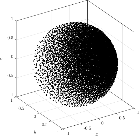
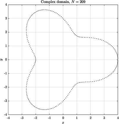
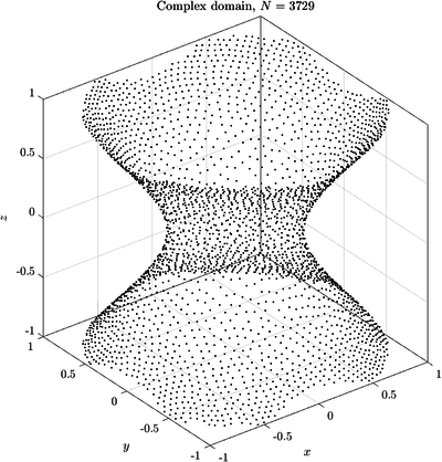
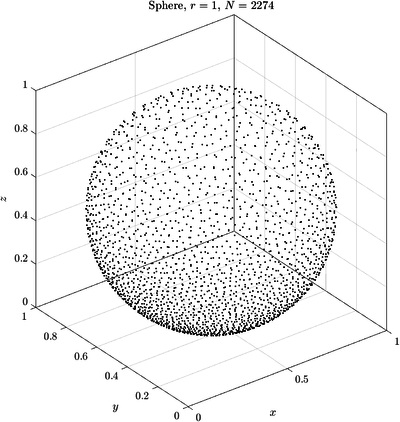
Examples of discretized 2D and 3D domains.

Computational times on a laptop computer, given as a rough reference. Filling a box with a hole with roughly 100 000 nodes.

• 2D, KDTree: 1.57 s, of which 5% is candidate generation, 85% is spatial queries and 4% is spatial inserts
• 2D, KDGrid: 0.35 s, of which 19% is candidate generation, 56% is spatial queries and 0.002% is spatial inserts
• 3D, KDTree: 7.87 s, of which 6% is candidate generation, 89% is spatial queries and 1% is spatial inserts
• 3D, KDGrid: 2.58 s, of which 16% is candidate generation, 70% is spatial queries and 0.001% is spatial inserts

Percentages vary slightly with N, with larger N increasing spatial query share by 2 percent points.

Filling parametric surfaces

The algorithm from the previous section can be modified to work on domain boundaries, for example curves in 2D and surfaces in 3D. Let $\partial \Omega$ be a domain boundary parametrized with a regular parametrization $\boldsymbol{r}: \Lambda \subset \mathbb{R}^{d - 1} \to \partial \Omega \subset \mathbb{R}^{d}$ and let $h(\boldsymbol{p})$ be our spacing function.

We can consider our problem as filling the domain $\Lambda$ in a way, that when its nodes are mapped by $\boldsymbol{r}$, they are approximately $h$ apart. The general logic of iteratively expanding nodes can thus stay the same, we only need to generate different candidates. Let $\boldsymbol{\lambda}_i \in \Lambda$ be the parameter we wish to expand. We want to generate candidates $\boldsymbol{\eta}_{i,j} \in H_i \subset \Lambda$ so that \begin{equation} ||\boldsymbol{r}(\boldsymbol{\eta}_{i,j}) - \boldsymbol{r}(\boldsymbol{\lambda}_i)|| = h(\boldsymbol{r}(\boldsymbol{\lambda}_i)). \end{equation} Let \begin{equation} \boldsymbol{\eta}_{i,j} = \boldsymbol{\lambda}_i + \alpha_{i, j} \vec{s}_{i,j}, \end{equation} where $\vec{s}_{i,j}$ is a unit vector and $\alpha_{i, j} > 0$. By using the first order Taylor's expansion we get \begin{align} h(\boldsymbol{r}(\boldsymbol{\lambda}_i)) &\approx ||\boldsymbol{r}(\boldsymbol{\lambda}_i) + \alpha_{i, j} \nabla \boldsymbol{r}(\boldsymbol{\lambda}_i) \vec s_{i, j} - \boldsymbol{r}(\boldsymbol{\lambda}_i)|| = \alpha_{i, j} ||\nabla \boldsymbol{r}(\boldsymbol{\lambda}_i) \vec s_{i, j}||, \\ \alpha_{i, j} &\approx \frac{h(\boldsymbol{r}(\boldsymbol{\lambda}_i))}{||\nabla \boldsymbol{r}(\boldsymbol{\lambda}_i) \vec s_{i, j}||}. \end{align} Therefore, our set of candidates for expansion of $\boldsymbol{\lambda}_i$ can be expressed as \begin{equation} H_i = \left\{ \boldsymbol{\lambda}_i + \frac{h(\boldsymbol{r}(\boldsymbol{\lambda}_i))}{||\nabla \boldsymbol{r}(\boldsymbol{\lambda}_i) \vec s_{i, j}||} \vec{s}_{i, j} ; \vec{s}_{i,j} \in S_i, \right\} \end{equation} where $S_i$ is a random discretization of a unit sphere.

Here are some examples of curves and surfaces filled with the described algorithm.

The described algorithm can also be used to fill surfaces defined by multiple patches, such as non-uniform rational basis spline (NURBS) models generated by Computer aided design (CAD) software. It is usually beneficial to discretize patch boundaries ($\partial \partial \Omega$) first, since it ensures no gaps of size between $h(\boldsymbol{p})$ and $2h(\boldsymbol{p})$ on patch boundaries.

Relaxation of the nodal distribution

To construct stable and reliable shape functions the support domains need to be non-degenerated [1], i.e. the distances between support nodes have to be balanced. Naturally, this condition is fulfilled in regular nodal distributions, but when working with complex geometries, the nodes have to be positioned accordingly. There are different algorithms designed to optimally fill the domain with different shapes [2, 3]. Here an intrinsic feature of the MLSM is used to take care of that problem. The goal is to minimize the overall support domain degeneration in order to attain stable numerical solution. In other words, a global optimization problem with the overall deformation of the local support domains acting as the cost function is tackled. We seek the global minimum by a local iterative approach. In each iteration, the computational nodes are translated according to the local derivative of the potential \begin{equation} \delta \b{p}\left( \b{p} \right)=-\sigma_{k}\sum\limits_{n=1}^{n}{\nabla }V\left( \mathbf{p}-\b{p}_n \right) \end{equation} where $V, n, \delta \b{p}, \b{p}_{n}$ and $\sigma_{k}$ stand for the potential, number of support nodes, offset of the node, position of n-th support node and relaxation parameter, respectively. After offsets in all nodes are computed, the nodes are repositioned as $\b{p}\leftarrow \b{p}+\delta \b{p}\left( \b{p} \right)$. Presented iterative process procedure begins with positioning of boundary nodes, which is considered as the definition of the domain, and then followed by the positioning of internal nodes.

The BasicRelax Engine supports two call types:

• with supplied distribution function relax(func), where it tries to satisfy the user supplied nodal density function. This can be achieved only when there is the total number of domain nodes the same as integral of density function over the domain. If there is too much nodes a volatile relax might occur. If there is not enough nodes the relax might become lazy. The best use of this mode is in combination with fillDistribution Engines.
• without distribution, where nodes always move towards less populated area. The relax magnitude is simply determined from Annealing factor and distance to the closest node. A simple and stable approach, however, note that this relax always converges towards uniformly distributed nodes.

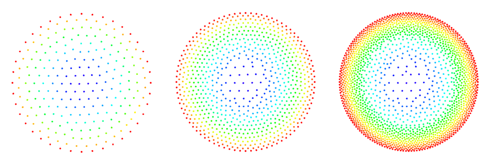
Example of filling and relaxing 2D domain can be found in below code snippet and Figure. Note the difference between relax without supplied distribution (right) and with supplied distribution (left). The quiver plot represents normal vectors in boundary nodes. More examples can be found in main repository under tests.

 1     double r = 0.25;
 2     CircleDomain<Vec2d> c({0.5, 0.5}, r);
 3 
 4     BasicRelax relax;
 5     relax.iterations(100).InitialHeat(1).FinalHeat(0).projectionType(1).numNeighbours(3);
 6     relax.boundaryProjectionThreshold(0.55);
 7     auto fill_density = [](Vec2d p) -> double {
 8         return (0.005 + (p[0] - 0.5) * (p[0] - 0.5) / 2 + (p[1] - 0.5) * (p[1] - 0.5) / 2);
 9     };
10 
11     c.fillUniformBoundaryWithStep(fill_density(Vec2d({r, 0.0})));
12     PoissonDiskSamplingFill fill_engine;
13 
14     fill_engine(c, fill_density);
15     relax(c);

[1] Lee CK, Liu X, Fan SC. Local muliquadric approximation for solving boundary value problems. Comput Mech. 2003;30:395-409.

[2] Löhner R, Oñate E. A general advancing front technique for filling space with arbitrary objects. Int J Numer Meth Eng. 2004;61:1977-91.

[3] Liu Y, Nie Y, Zhang W, Wang L. Node placement method by bubble simulation and its application. CMES-Comp Model Eng. 2010;55:89.

Refinement of the nodal distribution

Here we consider possible meshless refinement algorithms (sometimes also called adaptive cloud refinement). The refinement mechanisms we have so far studied include:

• refinement based on closest node distance
• refinement based on averaged (inter-)node distance
• refinement based on half-links

Here we only want to compare the quality of the refined grids and have not tied the refinement algorithm with a error indicator, thus we only study the node insertion process by refining the whole grid.

The refinement routine takes a range of nodes (e.g. a subregion of the domain) together with the refinement parameters and generates new nodes around the old ones. Special care must be taken with refinement of the boundary nodes. Points have to be selected on the actual boundary either analytically considering the geometry or with a numerical root finder such as bisection.

Problem description

To compare the node refinement mechanisms we study the process of reaction-diffusion in an infinite cylindrical catalyst pellet (infinite in the $z$-dimension). Since the pellet is infinite in one dimension this problem simplifies to a 2D problem (in the $xy$-plane). For a catalyst pellet of radius $R$ centered at $(x,y) = (0,0)$ and the reactant undergoing a first order reaction we must solve the equation \begin{equation} \b{\nabla}^2 C - {M_T}^2 C = 0, \end{equation} where $C$ is the concentration of the reactant, $M_T = R\sqrt{k/D}$ is known as Thiele's modulus and $k$ and $D$ represent the reaction rate constant and diffusivity of the reacting species. The boundary conditions for this problem is \[C(R) = C_s.\] The analytical solution can be found easily using cylindrical coordinates and is given by \begin{equation} \frac{C(r)}{C_S} = \frac{I_0(r M_T)}{I_0(R M_T)}, \end{equation} where $I_0(r)$ is the modified Bessel function of first kind (this function is available in the library Boost as well as scripting languages such as Python or MATLAB). The conversion from cartesian to cylindrical coordinates is given by \[r = \sqrt{x^2+y^2}.\]

Error indicators

To compare the quality of the refined meshes for the described problem case we look at different error criteria including the max norm $L_\infty$ defined as \begin{equation} L_\infty = \mathrm{max}_i \left|C_i^\mathrm{numerical} - C_i^\mathrm{analytical}\right|, \end{equation} the $L_2$ norm per node defined as \begin{equation} \bar{L_2} = \frac{\sqrt{\sum^N_{i = 1}\left(C_i^\mathrm{numerical} - C_i^\mathrm{analytical}\right)^2}}{N}, \end{equation} where $N$ is the number of nodes (and pertinent equations) in the domain.

We also measure the number of iterations required by the sparse BiCGSTAB solver to reach convergence and the estimated error of solving the system of equations.

Closest node

For a given node $\b{x}_0 = (x_0,y_0)$:

1. find the closest node $\b{x}_1 = (x_1,y_1)$
2. calculate the half distance between the two nodes \[d = |\b{x}_1 - \b{x}_0|/2\]
3. randomly select up to 6 (The case of 6 nodes is the limit since it produces a regular hexagon. In practice this never occurs due to the "monte carlo" node selection procedure.) new nodes on the circle with center $\b{x}_0$ and radius $d$ and simultaneously make sure their is a minimal inter-nodal distance $d$ between the new nodes.

For boundary points we first select 2 points that intersect with the boundary of the domain and only then points lying inside the domain. Due to geometrical constraints boundary points will usually end up with 3 new nodes (in case of straight boundaries we could end up with 4, which would be the previously discussed hexagon limit).

Figure 1: Refinement based on closest node approach (initial unrefined grid is on the left). In the second refinement step an erroneous point has appeared from an internal point that was too close to the boundary. Also noticable is clustering of points on the boundary.

Average radius

Input parameters: $f$ and $l_s$

For a given node $\b{x}_0$:

1. find the $l_s$ (an integer from 1 to 7) closest nodes
2. calculate the average distance $\bar{d}$ to the $l_s$ closest nodes
3. randomly select up to 6 new nodes on the circle with center $\b{x}_0$ and radius $f\cdot\bar{d}$ where $f$ is the radius fraction that lies between 0.2 (leads to clustering) and 0.8. Only allow nodes that are separated by the distance $f \cdot \bar{d}$.

(note that in case $l_s = 1$ and $f = 0.5$ the average radius mechanism becomes equal to the closest node refinement approach described above)

Figure 2: Refinement based on average radius approach (initial unrefined grid is on the left). The parameters are $l_s = 5$ closest nodes in average radius calculation and points placed at radius fraction $f = 0.5$.

Half-links

Input parameters: $l_s$, $d_m$

For a given node $\b{x}_0$:

1. find the $l_s$ (an integer from 1 to 7) closest nodes $\b{x}_i$
2. select new nodes in the middle of the segments $\b{x}_i - \b{x}_0$ only allowing points that are separated by the minimal distance $d_m$

(note also that in the 1D case the half-link and closest radius approach become the same)

The minimal distance $d_m$ is chosen as a fraction of the distance to the closest link, e.g. $d_m = f d$, where $f$ is the provided fraction and $d$ is the distance to the closest link.

Figure 3: Refinement based on half links (initial unrefined grid is on the left). The parameters are $l_s = 6$ and $d_m = 0.4 d$, where $d$ is the distance to the closest link.

Figure 4: Refinement based on half links with additional 10 step relax after refinement

After experimentation we noticed there are some inconsistencies when trying to refine structured point sets with this approach. The reason for these inconsistencies is that the boundary and internal points have a different number of "natural neighbours". For example in 2D on a square grid, the internal points have 8 neighbours, while boundary points have 5 neighbours. If we choose higher numbers e.g 9 links for an internal node, the 9th node might be any of the 4 nodes one shell further out that only differ at machine precision.

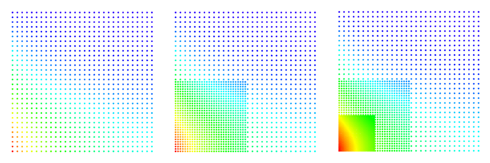
The figures below show some preliminary results of refinement based on half-links. For the circle domain relaxation was applied after the refinement.

Figure 5: Thermal diffusion in (convective) flow at a stagnation point (bottom left corner).

After the second refinement of the corner, the solver had difficulty converging to the solution. This was the result of a fixed size shape parameter in the shape functions of the node points. The shape functions have to be tailored to the local characteristic distance in the point set.

Figure 6: Reaction-diffusion in a cylinder catalyst. Two successive refinements have been applied for $r > 0.5$ and $r > 0.8$, where $r$ is the radial coordinate. The cylinder radius $R = 1$.$

Hybrid approach

A hybrid might give better distributions of the refined points. The half-link approach performs well at the boundaries while the distance approach gives less regular internal distributions. In any case it is suggested to perform a few more relaxation steps to equilibrate the mesh.

Figure 7: Refinement based on half links at the boundaries and closest distances for the internal nodes (initial unrefined grid is on the left). for the boundary nodes the parameters are $l_s = 7$ and $d_m = 0.5 d$, where $d$ is the distance to the closest link.