NURBS domains

Go back to Examples.

Medusa supports filling domains bounded by non-uniform rational basis splines (NURBS) curves and NURBS surfaces obtained as the tensor product of two NURBS curves. Note that Bézier curves and B-splines are special cases of NURBS curves.

See Positioning of computational nodes for details on node positioning algorithms.

Poisson equation with Dirichlet boundary conditions in 2D

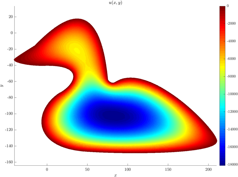
With Medusa, we can also solve partial differential equations on NURBS domains. Consider the solution of a simple 2D Poisson equation with Dirichlet boundary conditions\[ \begin{align*} \Delta u &= 20 &&\text{in } \Omega, \\ u &= 0 &&\text{on } \partial \Omega, \end{align*} \] where $\Omega$ is the interior of a NURBS curve defined piecewise. In this case, we will use a duck shaped curve composed of $8$ NURBS curve patches.

In Medusa, we represent NURBS patches as instances of NURBSPatch<vec_t, param_vec_t> class, where vec_t is the vector type of the ambient space (in this case Vec2d) and param_vec_t is the vector type of the parametric space (Vec1d for curves and Vec2d for surfaces). To construct an instance, its control points, weights, knot vector, and order $p$ must be given. In this case, we have a simple knot vector {0, 0, 0, 0, 1, 1, 1, 1}, all weights equal to $1$ and $p = 3$ (this means that our curves are Bézier curves). Control points will be calculated from pts. We will push all patches into one Range.

 1 // Points to be used in NURBS creation.
 2 Range<Vec2d> pts{{210, -132.5}, {205, -115}, {125, -35}, {85, -61}, {85, -61}, {85, -61},
 3                  {80, -65}, {75, -58}, {75, -58}, {65, 45}, {25, 25}, {-15, -16}, {-15, -16},
 4                  {-15, -16}, {-35, -28}, {-40, -32.375}, {-40, -32.375}, {-43, -35}, {-27, -40},
 5                  {-5, -40}, {-5, -40}, {50, -38}, {35, -65}, {15, -75}, {15, -75}, {-15, -95},
 6                  {-20, -140}, {45, -146}, {45, -146}, {95, -150}, {215, -150}, {210, -132.5}};
 7 
 8 // Calculate NURBS patches' control points, weights, knot vector and order.
 9 int p = 3;
10 Range<double> weights{1, 1, 1, 1};
11 Range<double> knot_vector{0, 0, 0, 0, 1, 1, 1, 1};
12 Range<NURBSPatch<Vec2d, Vec1d>> patches;
13 
14 for (int i = 0; i < 8; i++) {
15     Range<Vec2d> control_points;
16     for (int j = 0; j < 4; j++) {
17         control_points.push_back(pts[4 * i + j]);
18     }
19 
20     NURBSPatch<Vec2d, Vec1d> patch(control_points, weights, {knot_vector}, {p});
21     patches.push_back(patch);
22 }

Now, we can construct a NURBSShape<vec_t, param_vec_t> representing our NURBS curve from a Range of patches and fill it according to the spacing $h$. Spacing can also be given in the form of a spacing function, see Parametric domains.

1 // Create NURBS shape from a range of patches.
2 NURBSShape<Vec2d, Vec1d> shape(patches);
3 
4 // Fill the domain.
5 double h = 0.5;
6 DomainDiscretization<Vec2d> domain = shape.discretizeBoundaryWithStep(h);

After that, we can fill the interior of the domain in the usual way.

1 GeneralFill<Vec2d> gf;
2 gf(domain, h);

Finally, we translate the partial differential equations of our problem into code and solve the problem, as in other examples.

 1 // Construct the approximation engine.
 2 int m = 2;  // basis order
 3 Monomials<Vec2d> mon(m);
 4 RBFFD<Polyharmonic<double, 3>, Vec2d> approx({}, mon);
 5 
 6 // Find support for the nodes.
 7 int N = domain.size();
 8 domain.findSupport(FindClosest(mon.size()));
 9 
10 // Compute the shapes (we only need the Laplacian).
11 auto storage = domain.computeShapes<sh::lap>(approx);
12 
13 Eigen::SparseMatrix<double, Eigen::RowMajor> M(N, N);
14 Eigen::VectorXd rhs(N);
15 rhs.setZero();
16 M.reserve(storage.supportSizes());
17 
18 // Construct implicit operators over our storage.
19 auto op = storage.implicitOperators(M, rhs);
20 
21 for (int i : domain.interior()) {
22     // set the case for nodes in the domain
23     op.lap(i) = 20.0;
24 }
25 for (int i : domain.boundary()) {
26     // enforce the boundary conditions
27     op.value(i) = 0.0;
28 }
29 
30 Eigen::BiCGSTAB<decltype(M), Eigen::IncompleteLUT<double>> solver;
31 solver.compute(M);
32 ScalarFieldd u = solver.solve(rhs);

Here is the plot of $u(x, y)$.

The whole example can be found as poisson_NURBS_2D.cpp along with the plot script that can be run by Matlab or Octave poisson_NURBS_2D_2D.m.