Poisson's equation

Dirtchlet boundary conditions

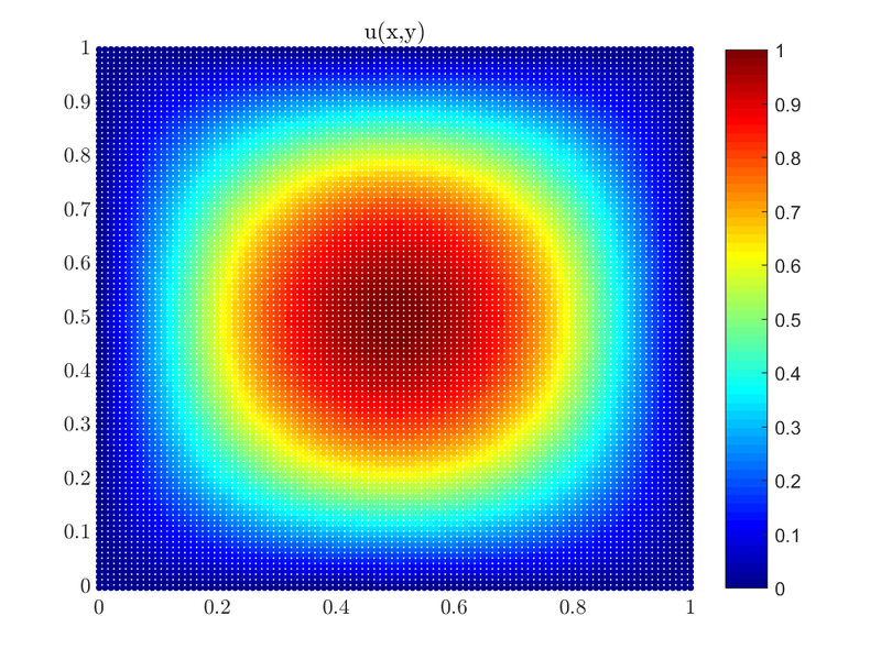
It is fitting that examples start with a simple case, and we will gradually make our way towards more complicated cases with different domain shapes, boundary conditions and approximation types. Consider the solution of the 2D Poisson equation on a unit square with Dirichlet boundary conditions\[ \begin{align*} \Delta u &= f &&\text{in } \Omega, \\ u &= 0 &&\text{on } \partial \Omega, \end{align*} \] where $u(x,y)$ is the solution to the problem, $\Omega = [0, 1] \times [0, 1]$ and in the case we will consider $f(x,y) = -2\pi^2\sin(\pi x)\sin(\pi y)$, as it makes for a simple solution $u(x,y) = \sin(\pi x)\sin(\pi y)$.

First, we construct our domain and discretize it, then find support (neighborhood) for each node.

1 BoxShape<Vec2d> box(0.0, 1.0);
2 double dx = 0.01;
3 DomainDiscretization<Vec2d> domain = box.discretizeWithStep(dx);
4 
5 int N = domain.size();
6 domain.findSupport(FindClosest(9));

We constructed a box shape, discretized it with a constant step dx (both inside and the boundary) and choose the closest 9 nodes of each node as its support. The next step is to construct our approximation engine. Simply put, approximation engines are classes responsible for computing shape functions for given operator and points. While many different setups are supported in Medusa we will start off simple, with an approximation that reproduces standard Finite Difference method.

1 int m = 2
2 WLS<Monomials<Vec2d>, NoWeight<Vec2d>, ScaleToFarthest> wls(Monomials<Vec2d>::tensorBasis(m));

We constructed a WLS engine using monomial tensor basis of order 2. Finally, we write the equations for our problem by directly translating the mathematical formulation above into code.

1 for (int i : domain.interior()) {
2     double x = domain.pos(i, 0);
3     double y = domain.pos(i, 1);
4     op.lap(i) = -2*PI*PI*std::sin(PI*x)*std::sin(PI*y);
5 }
6 for (int i : domain.boundary()) {
7     op.value(i) = 0.0;
8 }

Here is the plot of the solution $u(x, y)$.

TODO Popravi sliko

The whole example can be found as poisson_implicit_dirichlet_2D.cpp along with the plot script that can be run by Matlab or Octave poisson_implicit_dirichlet_2D.m. Same goes for a similar cases solved in 1D and 3D and their respective plot scripts.

Mixed boundary conditions

We can obtain the solution to the above problem by solving it on just a quarter of the original domain and using mixed boundary conditions. By using Dirichlet boundary conditions on the bottom and the left side of the square domain, and Neumann boundary conditions on the right and upper side of the domain we are effectively solving the same problem but on a quarter of the domain. Our problem is now\[ \begin{align*} \Delta u &= f &&\text{in } \Omega, \\ u &= 0 &&\text{on } \partial \Omega_1 \cup \Omega_3,\\ \frac{du}{d \b{\hat{n}}} &= 0 &&\text{on } \partial \Omega_2 \cup \Omega_4 \end{align*} \]

Where $\partial \Omega_1$, $\partial \Omega_2$, $\partial \Omega_3$ and $\partial \Omega_4$ are left, right, bottom and top boundary respectively. The domain is $\Omega = [0, 0.5] \times [0, 0.5]$, and $\frac{du}{d \b{\hat{n}}}$ is the normal derivative (on the boundary).

When constructing approximation engines, there are a lot of different options, you can choose between different basis functions, weights, scale functions and each setup comes with its advantages and disadvantages. Some might work for certain problems and some might not. When writing the examples we tried to present the reader with as many different options as possible.

Let us solve the problem using Gaussian RBF (Radial Basis Functions) instead of Monomials:

1     // shape = 30
2     // m = 9
3     WLS<Gaussians<Vec2d>, NoWeight<Vec2d>, ScaleToFarthest,
4             Eigen::LLT<Eigen::MatrixXd>> wls({9, 30});

While the case is the same for the nodes inside the domain, we need to change the boundary conditions:

 1     int BOTTOM = -3;
 2     int TOP = -4;
 3     int LEFT = -1;
 4     int RIGHT = -2;
 5 
 6     for (int i : (domain.types() == LEFT) + (domain.types() == BOTTOM)) {
 7         op.value(i) = 0.0;  // Dirichlet boundary conditions on the left and bottom edge of the box
 8     }
 9     for (int i : (domain.types() == TOP) + (domain.types() == RIGHT)) {
10         // Neumann boundary conditions on upper and right edge of the box
11         op.neumann(i, domain.normal(i)) = 0.0;
12     }

When solving a PDE implicitly a system of equations needs to be solved to obtain the solution. For this, we use Eigen.

1     Eigen::BiCGSTAB<decltype(M), Eigen::IncompleteLUT<double>> solver;
2     solver.compute(M);
3     ScalarFieldd u = solver.solve(rhs);

Matrix M and rhs are the sparse matrix and vector in which we wrote (with the help of Medusa) the system of equations that when solved gives us an approximate solution of our problem. We solve the system using an Eigen linear equation solver, in this case, the BiCGStab algorithm with ILUT preconditioning. The solution is plotted bellow:

Full Neumann boundary conditions

TODO