De Vahl Davis natural convection test
Click here to return back to Fluid Mechanics
Contents
Intro
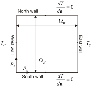
The classical de Vahl Davis benchmark test is defined for the natural convection of the air ($\Pr =0.71$) in the square closed cavity (${{\text{A}}_{\text{R}}}=1$). The only physical free parameter of the test remains the thermal Rayleigh number. In the original paper [1] de Vahl Davis tested the problem up to the Rayleigh number ${{10}^{6}}$, however in the latter publications, the results of more intense simulations were presented with the Rayleigh number up to ${{10}^{8}}$. Lage and Bejan [2] showed that the laminar domain of the closed cavity natural convection problem is roughly below $\text{Gr1}{{\text{0}}^{9}}$. It was reported [3, 4] that the natural convection becomes unsteady for $\text{Ra}=2\cdot {{10}^5}$. Here we present a MLSM solution of the case.
\begin{equation} \text{Ra}\text{=}\,\frac{\left| \mathbf{g} \right|{{\beta }_{T}}\left( {{T}_{H}}-{{T}_{C}} \right){{\Omega }_{H}}^{3}{{\rho }^{2}}{{c}_{p}}}{\lambda \mu } \end{equation} \begin{equation} \text{Pr}=\frac{\mu {{c}_{p}}}{\lambda } \end{equation}
[1] de Vahl Davis G. Natural convection of air in a square cavity: a bench mark numerical solution. Int J Numer Meth Fl. 1983;3:249-64.
[2] Lage JL, Bejan A. The Ra-Pr domain of laminar natural convection in an enclosure heated from the side. Numer Heat Transfer. 1991;A19:21-41.
[3] Janssen RJA, Henkes RAWM. Accuracy of finite-volume disretizations for the bifurcating natural-convection flow in a square cavity. Numer Heat Transfer. 1993;B24:191-207.
[4] Nobile E. Simulation of time-dependent flow in cavities with the additive-correction multigrid method, part II: Apllications. Numer Heat Transfer. 1996;B30:341-50.
Code
Full examples can be found under the examples in the code repository Main Page).
Explicit ACM method with CBS looks
 1     v2[boundary] = vec_t{0.0, 0.0};
 2     T2[left] = O.T_cold;
 3     T2[right] = O.T_hot;
 4     //Time stepping
 5     for (int step = 0; step <= O.t_steps; ++step) {
 6         for (int i_count = 1; i_count < _MAX_ITER_; ++i_count) {
 7             // Navier Stokes
 8             for (auto c : interior) {
 9                 v2[c] = v1[c] + O.dt * (-1 / O.rho * op.grad(P1, c)
10                                         + O.mu / O.rho * op.lap(v1, c)
11                                         - op.grad(v1, c) * v1[c]
12                                         + O.g * (1 - O.beta * (T1[c] - O.T_ref)));
13             }
14
15             //Speed of sound
16             Range<scal_t> norm = v2.map([](const vec_t& p) { return p.norm(); });
17             scal_t C = O.dl * std::max(*std::max_element(norm.begin(), norm.end()), O.v_ref);
18             // Mass continuity
19             Range<scal_t> div_v;
20             for (auto c:all) {
21                 div_v[c] = op.div(v2, c);
22                 P2[c] = P1[c] - C * C * O.dt * O.rho * div_v[c] +
23                         O.dl2 * C * C * O.dt * O.dt * op.lap(P1, c);
24             }
25             P1.swap(P2);
26         }
27
28         //heat transport
29         for (auto c : interior) {
30             T2[c] = T1[c] + O.dt * O.lam / O.rho / O.c_p * op.lap(T1, c) -
31                     O.dt * v1[c].transpose() * op.grad(T1, c);
32         }
33         for (auto c : top) T2[c] = op.neumann(T2, c, vec_t{0, -1}, 0.0);
34         for (auto c : bottom) T2[c] = op.neumann(T2, c, vec_t{0, 1}, 0.0);
35     }
Explicit pressure correction
The solution of heat equation is the same as in above example
 1     for (int step = 0; step <= O.t_steps; ++step) {
 2
 3         // Explicit Navier-Stokes computed on whole domain, including boundaries
 4         // without pressure
 5         for (int c:all) {
 6             v_2[c] = v_1[c] + O.dt (
 7                                    O.mu / O.rho * op.lap(v_1, c)
 8                                     - op.grad(v_1, c) * v_1[c]
 9                                     + O.g * (1 - O.beta * (T_1[c] - O.T_ref)));
10         }
11         // Pressure correction
12         VecXd rhs_pressure(N + 1, 0); //Note N+1, +1 stands for regularization equation
13         rhs_pressure(N) = 0; // = 0 part of the regularization equation
14         for (int i:interior) rhs_pressure(c) = O.rho / O.dt * op.div(v_2, c);
15
16         for (int i: boundary) rhs_pressure(c) = O.rho / O.dt * v_2[c].dot(domain.normal(c));
17         VecXd solution = solver_p.solve(rhs_pressure);
18         alpha = solution[N];
19         VecXd P_c = solution.head(N);
20         for ( int i = interior) v_2[c] -=  O.dt / O.rho * op.grad(P_c, c);
21
22         v_2[boundary] = 0; // force boundary conditions
23 }
Full implicit
 1 for (int step = 0; step <= O.t_steps_i; ++step) {
 2         time_1 = std::chrono::high_resolution_clock::now();
 3         // NAVIER STOKES
 4         M_velocity = mat_t(2 * N, 2 * N);
 5         // system
 6         M_velocity.reserve(Range<int>(2 * N, O.n));
 7         for (int i : interior) {
 8             op.valuevec(M_velocity, i, 1 / O.dt_i);
 9             op.lapvec(M_velocity, i, -O.mu / O.rho);
10             // op.gradvec(M_velocity, i, v_1[i]);
11         }
12         for (int i : boundary) op.valuevec(M_velocity, i, 1); //sets velocity to 0
13
14         M_velocity.makeCompressed();
15         solver_v.compute(M_velocity);
16         // solution
17         Range <vec_t> rhs_vec(domain.size(), 0);
18         for (int i : interior) {
19             rhs_vec[i] = -1 / O.rho * op.grad(P, i) +
20                          v_1[i] / O.dt_i
21                          + O.g * (1 - O.beta * (T[i] - O.T_ref));
22         }
23         // for (int i:top) rhs_vec[i] = vec_t{0,1};
24
25         v_2 = reshape<2>(solver_v.solveWithGuess(reshape(rhs_vec), reshape(v_1)));
26         // END OF NAVIER STOKES
27
28         // PRESSURE CORRECTION
29         VecXd rhs_pressure(N + 1, 0); //Note N+1, +1 stands for regularization equation
30         rhs_pressure(N) = 0; // = 0 part of the regularization equation
31         double alpha;
32         for (int i : interior) rhs_pressure(i) = O.rho / O.dt_i * op.div(v_2, i);
33         for (int i : boundary) rhs_pressure(i) = O.rho / O.dt * v_2[i].dot(domain.normal(i));
34
35         VecXd solution = solver_p.solve(rhs_pressure);
36         alpha = solution[N];
37         VecXd P_c = solution.head(N);
38         // apply velocity correction
39         for (int i : interior) {
40             v_2[i] -= O.dl * O.dt_i / O.rho * op.grad(P_c, i);
41         }
42         P += O.dl * P_c;
43         // enforce velocity BC
44         // v_2[boundary] = 0;
45         // END OF PRESSURE CORRECTION
46
47         // HEAT TRANSPORT
48         M_temperature = mat_t(N, N);
49         Range<int> per_row(N, O.n);
50         M_temperature.reserve(per_row);
51         // outer boundary dirichlet BC
52         for (int i : top) op.neumann_implicit(M_temperature, i, domain.normal(i), 1);
53         for (int i : bottom) op.neumann_implicit(M_temperature, i, domain.normal(i), 1);
54         for (int i : left) op.value(M_temperature, i, 1.0);
55         for (int i : right) op.value(M_temperature, i, 1.0);
56         // heat transport in air
57         for (int i : interior) {
58             op.value(M_temperature, i, 1.0);                          // time dependency
59             op.lap(M_temperature, i, -O.dt_i * O.lam / O.rho / O.c_p);  //laplace in interior
60             op.grad(M_temperature, i, O.dt * v_2[i]);
61         }
62         M_temperature.makeCompressed();
63         solver_T.compute(M_temperature);
64
65         VectorXd rhs = VectorXd::Zero(N);
66         for (int i : interior) rhs(i) = T(i);
67         for (int i : top) rhs(i) = 0;
68         for (int i : bottom) rhs(i) = 0;
69         for (int i : left) rhs(i) = O.T_hot;
70         for (int i : right) rhs(i) = O.T_cold;
71         T = solver_T.solveWithGuess(rhs, T);
72         // END OF HEAT TRANSPORT
73         v_1.swap(v_2);
74 }
Results
Comparison of MLSM solution with reference data
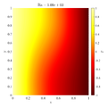
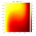
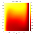
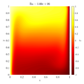
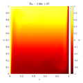
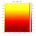
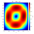
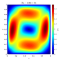
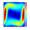
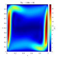
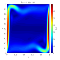
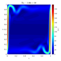
Following video shows evolution of temperature and velocity magnitude for the $Ra=10^8$ case.
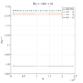
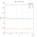
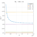
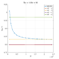
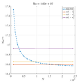
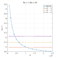
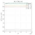
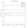
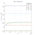
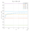
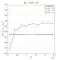
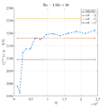
In below galley you can find temperature contour plots, velocity magnitude contour plots, v_max and average hot side Nusselt number convergence behavior. The reference values are from:
- [a] de Vahl Davis G. Natural convection of air in a square cavity: a bench mark numerical solution. Int J Numer Meth Fl. 1983;3:249-64.
- [b] Sadat H, Couturier S. Performance and accuracy of a meshless method for laminar natural convection. Numer Heat Transfer. 2000;B37:455-67.
- [c] Wan DC, Patnaik BSV, Wei GW. A new benchmark quality solution for the buoyancy-driven cavity by discrete singular convolution. Numer Heat Transfer. 2001;B40:199-228.
- [d] Šarler B. A radial basis function collocation approach in computational fluid dynamics. CMES-Comp Model Eng. 2005;7:185-93.
- [e] Kosec G, Šarler B. Solution of thermo-fluid problems by collocation with local pressure correction. Int J Numer Method H. 2008;18:868-82.
Quick comparison of explicit ACM, explicit pressure correction, and implicit methods
This section is not completed yet!
In below images you can see quick comparison of explicit stepping with ACM p-v coupling (EACM) [row 1 col 1], explicit stepping with pressure correction p-v coupling (EPC) [row 1 col 2], and fully implicit stepping with pressure correction p-v coupling (IPV) with 1000, 100, 10, 1 times bigger time step [rows 2-3] in comaprison to the EACM adn EPC. EACM and EPC agree well, also the implicit solution converges towards the EACM and EPC but only with the same time step as in explicit approaches.
