De Vahl Davis natural convection test
Click here to return back to Fluid Mechanics
Intro
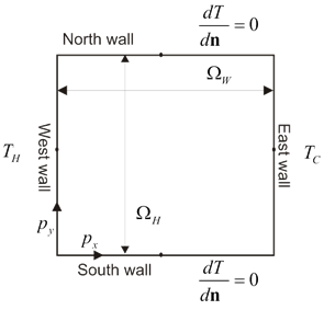
The classical de Vahl Davis benchmark test is defined for the natural convection of the air ($\Pr =0.71$) in the square closed cavity (${{\text{A}}_{\text{R}}}=1$). The only physical free parameter of the test remains the thermal Rayleigh number. In the original paper [1] de Vahl Davis tested the problem up to the Rayleigh number ${{10}^{6}}$, however in the latter publications, the results of more intense simulations were presented with the Rayleigh number up to ${{10}^{8}}$. Lage and Bejan [2] showed that the laminar domain of the closed cavity natural convection problem is roughly below $\text{Gr1}{{\text{0}}^{9}}$. It was reported [3, 4] that the natural convection becomes unsteady for $\text{Ra}=2\cdot {{10}^5}$. Here we present a MLSM solution of the case.
\begin{equation} \text{Ra}\text{=}\,\frac{\left| \mathbf{g} \right|{{\beta }_{T}}\left( {{T}_{H}}-{{T}_{C}} \right){{\Omega }_{H}}^{3}{{\rho }^{2}}{{c}_{p}}}{\lambda \mu } \end{equation} \begin{equation} \text{Pr}=\frac{\mu {{c}_{p}}}{\lambda } \end{equation}
[1] de Vahl Davis G. Natural convection of air in a square cavity: a bench mark numerical solution. Int J Numer Meth Fl. 1983;3:249-64.
[2] Lage JL, Bejan A. The Ra-Pr domain of laminar natural convection in an enclosure heated from the side. Numer Heat Transfer. 1991;A19:21-41.
[3] Janssen RJA, Henkes RAWM. Accuracy of finite-volume disretizations for the bifurcating natural-convection flow in a square cavity. Numer Heat Transfer. 1993;B24:191-207.
[4] Nobile E. Simulation of time-dependent flow in cavities with the additive-correction multigrid method, part II: Apllications. Numer Heat Transfer. 1996;B30:341-50.
Code
The snippet of the openMP parallel MLSM code for an explicit ACM method with CBS looks like: (full examples, including implicit versions, can be found under the examples in the code repository Main Page).
 1     v2[boundary] = vec_t{0.0, 0.0};
 2     T2[left] = O.T_cold;
 3     T2[right] = O.T_hot;
 4     //Time stepping
 5     for (int step = 0; step <= O.t_steps; ++step) {
 6         for (int i_count = 1; i_count < _MAX_ITER_; ++i_count) {
 7             // Navier Stokes
 8             for (auto c : interior) {
 9                 v2[c] = v1[c] + O.dt * (-1 / O.rho * op.grad(P1, c)
10                                         + O.mu / O.rho * op.lap(v1, c)
11                                         - op.grad(v1, c) * v1[c]
12                                         + O.g * (1 - O.beta * (T1[c] - O.T_ref)));
13             }
14
15             //Speed of sound
16             Range<scal_t> norm = v2.map([](const vec_t& p) { return p.norm(); });
17             scal_t C = O.dl * std::max(*std::max_element(norm.begin(), norm.end()), O.v_ref);
18             // Mass continuity
19             Range<scal_t> div_v;
20             for (auto c:all) {
21                 div_v[c] = op.div(v2, c);
22                 P2[c] = P1[c] - C * C * O.dt * O.rho * div_v[c] +
23                         O.dl2 * C * C * O.dt * O.dt * op.lap(P1, c);
24             }
25             P1.swap(P2);
26         }
27
28         //heat transport
29         for (auto c : interior) {
30             T2[c] = T1[c] + O.dt * O.lam / O.rho / O.c_p * op.lap(T1, c) -
31                     O.dt * v1[c].transpose() * op.grad(T1, c);
32         }
33         for (auto c : top) T2[c] = op.neumann(T2, c, vec_t{0, -1}, 0.0);
34         for (auto c : bottom) T2[c] = op.neumann(T2, c, vec_t{0, 1}, 0.0);
35     }
Snippet of code for explicit pressure correction scheme. Note that the solution of heat equation is the same as in above example
 1     for (int step = 0; step <= O.t_steps; ++step) {
 2         time_1 = std::chrono::high_resolution_clock::now();
 3         // Explicit Navier-Stokes computed on whole domain, including boundaries
 4         // without pressure -- Fraction step
 5         int i;
 6         #pragma omp parallel for private(i) schedule(static)
 7         for (i = 0; i < all.size(); ++i) {
 8             int c = i; //interior[i];
 9             v_2[c] = v_1[c] + O.dt (
10                                    O.mu / O.rho * op.lap(v_1, c)
11                                     - op.grad(v_1, c) * v_1[c]
12                                     + O.g * (1 - O.beta * (T_1[c] - O.T_ref)));
13         }
14         // Pressure correction
15         VecXd rhs_pressure(N + 1, 0); //Note N+1, +1 stands for regularization equation
16         rhs_pressure(N) = 0; // = 0 part of the regularization equation
17         #pragma omp parallel for private(i) schedule(static)
18         for (i = 0; i < interior.size(); ++i) {
19             int c = interior[i];
20             rhs_pressure(c) = O.rho / O.dt * op.div(v_2, c);
21         }
22         #pragma omp parallel for private(i) schedule(static)
23         for (i = 0; i < boundary.size(); ++i) {
24             int c = boundary[i];
25             rhs_pressure(c) = O.rho / O.dt * v_2[c].dot(domain.normal(c));
26         }
27
28         VecXd solution = solver_p.solve(rhs_pressure);
29         alpha = solution[N];
30         VecXd P_c = solution.head(N);
31
32         // veclocity correction due to the pressure correction
33         #pragma omp parallel for private(i) schedule(static)
34         for ( int i = interior) v_2[c] -=  O.dt / O.rho * op.grad(P_c, c);
35
36         v_2[boundary] = 0; // force boundary conditions
Results
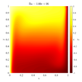
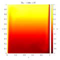
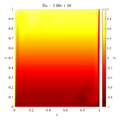
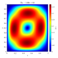
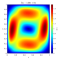
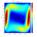
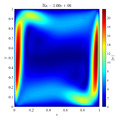
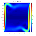
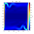
Following video shows evolution of temperature and velocity magnitude for the $Ra=10^8$ case.
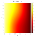
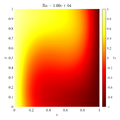
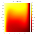
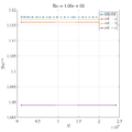
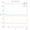
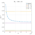
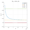
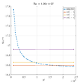
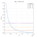
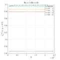
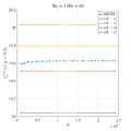
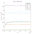
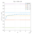
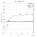
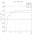
In below galley you can find temperature contour plots, velocity magnitude contour plots, v_max and average hot side Nusselt number convergence behavior. The reference values are from:
- [a] de Vahl Davis G. Natural convection of air in a square cavity: a bench mark numerical solution. Int J Numer Meth Fl. 1983;3:249-64.
- [b] Sadat H, Couturier S. Performance and accuracy of a meshless method for laminar natural convection. Numer Heat Transfer. 2000;B37:455-67.
- [c] Wan DC, Patnaik BSV, Wei GW. A new benchmark quality solution for the buoyancy-driven cavity by discrete singular convolution. Numer Heat Transfer. 2001;B40:199-228.
- [d] Šarler B. A radial basis function collocation approach in computational fluid dynamics. CMES-Comp Model Eng. 2005;7:185-93.
- [e] Kosec G, Šarler B. Solution of thermo-fluid problems by collocation with local pressure correction. Int J Numer Method H. 2008;18:868-82.
