Convection Diffusion equation

Before moving to more complex numerical examples, preliminary tests are done on a case with a known closed form solution. As in all the previous examples, we use the diffusion equation for a test case. The main purpose of this section is basic evaluation of mesh based against meshless methods, as well as strong form against weak form methods. More specific analyses and performance tests are presented in Chapter \ref{cases}.

\section{Diffusion equation}

\index{Diffusion equation} A 2D diffusion equation in its dimensionless form is considered: \begin{align} %??? brezdimenzijska oblika nima c \frac{\partial u}{\partial t} - \nabla^2u = q, & \qquad (x, y)\in \Omega, \label{eq.diffu}\\ % \frac{\partial u(x,y,t)}{\partial t} = \nabla^2 u(x,y,t), & \qquad (x, y)\in \Omega, \label{eq.diffusion}\\ u(x,y,t) = \overline{u}(x,y,t), & \qquad (x,y) \in \Gamma_D,\label{eq.bc_diffu}\\ u(x,y,t),_n = \overline{g}(x,y,t), & \qquad (x,y) \in \Gamma_N, \label{eq.mixed.bc_diffu}\\ u(x,y,t) = u_0, & \qquad t=0,\label{eq.ic_diffu} \end{align} where $(x,y)$ are spatial coordinates, $t$ is time, $u(x, y, t)$ is the unknown solution, $ \Omega$, and $ \Gamma_D$ and $ \Gamma_N$ are the global domain with Dirichlet boundary and Neumann boundary, $\overline{u}$ and $\overline{g}$ are the prescribed Dirichlet and Neumann boundary values and $u(x,y,0)=u_0$ is the known initial condition.

Boring 1D case

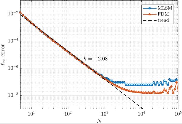
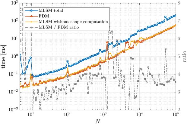
First, a simple one dimensional case is tackled to assess basic properties of presented solution method. Consider the problem \begin{align} u''(x) &= \sin(x), \quad x \in (0, 1) \nonumber \\ u(0) &= 0 \label{eq:neu1d} \\ u'(1) &= 0 \nonumber \end{align} with analytical solution \begin{equation} u(x) = x \cos 1 - \sin x. \end{equation} We solve the problem with MLSM using 3 support nodes and 3 monomials $\{1, x, x^2\}$ as basis functions on a regularly distributed nodes. This setup of MLSM is theoretically equivalent to the Finite Difference Method (FDM) and therefore it is worth implementing also standard FDM to compare results and execution times. The error between the actual solution $u$ and the approximate solution $\hat{u}$ is measured in $\ell_\infty$ norm, \begin{equation} \|u - \hat{u}\|_{\ell_\infty} = \max_{x\in X} | u(x) - \hat{u}(x)|, \label{eq:linf-err} \end{equation} where $X$ is the set of all points in the domain. The problem can be solved with below code.

1 for (int i : domain.internal()) {
2     op.lap(M, i, 1.0);  // Equation.
3     rhs(i) = std::sin(domain.positions[i][0]);
4 }
5 op.value(M, left, 1.0); // Left BC.
6 op.neumann(M, right, {1}, 1.0);  // Right BC.
7 VectorXd solution = M.lu().solve(rhs);