Positioning of computational nodes
Although the meshless methods do not require any topological relations between nodes and even randomly distributed nodes could be used, it is well-known that using regularly distributed nodes leads to more accurate and more stable results. So despite meshless seeming robustness regarding the nodal distribution, a certain effort has to be invested into the positioning of the nodes and following discussion, to some extent, deals with this problem. In a following discussion we want to form set of algorithms that can cover arbitrary domain in n dimensions with nodes that can be further used to solve systems of PDEs. We start with algorithms for filling the domain with nodes. Second set of algorithms is denoted to improving of the nodal distributions and a last set of algorithms deals with the refinement of the nodal distribution. The algorithms can of course be combined.
Filling domain with nodes
The goal is to fill arbitrary domain, which we can ask if position $\b{p}$ is in the domain our outside, with nodes following the given target density function $\rho(\b{p})$.
We start with a simple algorithm based on Poisson Disk Sampling (PDS) that results in a relatively tightly packed distribution of nodes. What we do is:
- Randomly select a node within the domain.
- Add N (depending on the dimensionality of the space) nodes on circle/sphere around that node.
- Randomly select one of just added nodes and repeat adding.
- Each time check if any of new nodes violates minimal distance criterion, i.e. if it is positioned to close to any of the existing nodes.
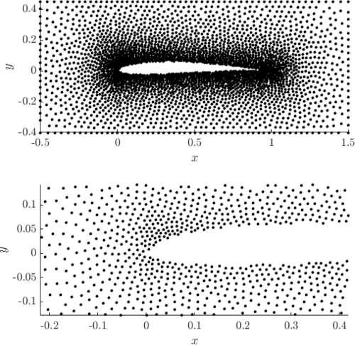
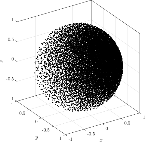
Examples of PDS discretized irregular domains in 2D (first code snippet, left image) and in 3D (second code snipper, right image) can be found below.
 1     // setup
 2     PoissonDiskSamplingFill fill_engine;
 3     fill_engine.iterations(1000000).optim_after(1000).use_MC(true).proximity_relax(0.8);
 4     // create test domain
 5     RectangleDomain<Vec2d> domain({0, 0}, {1.2, 1.5});
 6     CircleDomain<Vec2d> o1({0.4, 0.4}, 0.25);
 7     domain.subtract(o1);
 8     // define density function
 9     auto fill_density = [](Vec2d p)->double{
10         return (std::pow(p[0]/10, 2) + 0.01);
11     };
12     fill_engine(domain, fill_density);
 1 PoissonDiskSamplingFill fill_engine;
 2     // setup
 3     PoissonDiskSamplingFill fill_engine;
 4     fill_engine.iterations(1000000).optim_after(1000).use_MC(true).proximity_relax(0.8);
 5     // create test domain
 6     RectangleDomain<Vec3d> domain({0, 0, 0}, {1.2, 1.5, 1.1});
 7     CircleDomain<Vec3d> o1({0, 0, 0}, 0.5);
 8     domain.subtract(o1);
 9     // define target density
10     auto fill_density = [](Vec3d p)->double{
11         return (std::pow(p[0]/10 + p[1]/10 + p[2]/10, 2) + 0.025);
12     };
13     fill_engine(domain, fill_density);
Examples of PDS discretized in 2D and in 3D generated with above code.
Relaxation of the nodal distribution
To construct stable and reliable shape functions the support domains need to be non-degenerated [1], i.e. the distances between support nodes have to be balanced. Naturally, this condition is fulfilled in regular nodal distributions, but when working with complex geometries, the nodes have to be positioned accordingly. There are different algorithms designed to optimally fill the domain with different shapes [2, 3]. Here an intrinsic feature of the MLSM is used to take care of that problem. The goal is to minimize the overall support domain degeneration in order to attain stable numerical solution. In other words, a global optimization problem with the overall deformation of the local support domains acting as the cost function is tackled. We seek the global minimum by a local iterative approach. In each iteration, the computational nodes are translated according to the local derivative of the potential \begin{equation} \delta \b{p}\left( \b{p} \right)=-\sigma_{k}\sum\limits_{n=1}^{N_S}{\nabla }V\left( \mathbf{p}-\b{p}_n \right) \end{equation}
$\alpha$
where $V, \delta \b{p}, \b{p}_{n}}$
and $\sigma_{k}$ stand for the potential, offset of the node, position of n-th support node and relaxation parameter, respectively. After offsets in all nodes are computed, the nodes are repositioned as $\b{p}\leftarrow \b{p}+\delta \b{p}\left( \b{p} \right)$. Presented iterative process procedure begins with positioning of boundary nodes, which is considered as the definition of the domain, and then followed by the positioning of internal nodes.
[1] Lee CK, Liu X, Fan SC. Local muliquadric approximation for solving boundary value problems. Comput Mech. 2003;30:395-409. [2] Löhner R, Oñate E. A general advancing front technique for filling space with arbitrary objects. Int J Numer Meth Eng. 2004;61:1977-91. [3] Liu Y, Nie Y, Zhang W, Wang L. Node placement method by bubble simulation and its application. CMES-Comp Model Eng. 2010;55:89.

