Solving sparse systems

There are many methods available for solving sparse systems. We compare some of them here.

Figure 1: Matrix of the discretized PDE.

Mathematica has the following methods available (https://reference.wolfram.com/language/ref/LinearSolve.html#DetailsAndOptions)

• direct: banded, cholesky, multifrontal (direct sparse LU)
• iterative: Krylov

Matlab has the following methods:

• direct: https://www.mathworks.com/help/matlab/ref/mldivide.html#bt42omx_head
• iterative: https://www.mathworks.com/help/matlab/math/systems-of-linear-equations.html#brzoiix, including bicgstab, gmres

Eigen has the following methods: (https://eigen.tuxfamily.org/dox-devel/group__TopicSparseSystems.html)

• direct: sparse LU
• iterative: bicgstab, cg

Solving a simple sparse system $A x = b$ for steady space of heat equation in 1d with $n$ nodes, results in a matrix shown in Figure 1.

The following timings of solvers are given in seconds:

$n = 10^6$	Matlab	Mathematica	Eigen
Banded	0.16	0.28	0.04
SparseLU	/	1.73	0.82
BICGStab / Krylov	0.33	0.39	0.53

Incomplete LU preconditioner was used for BICGStab. Without the preconditioner BICGStab does not converge.

Parallel execution

BICGStab can be run in parallel, as explain in the general parallelism: https://eigen.tuxfamily.org/dox/TopicMultiThreading.html, and specifically

"When using sparse matrices, best performance is achied for a row-major sparse matrix format.
Moreover, in this case multi-threading can be exploited if the user code is compiled with OpenMP enabled".

Eigen uses number of threads specified my OopenMP, unless Eigen::setNbThreads(n); was called. Minimal working example:

Figure 2: Memory and CPU usage. C stands for construction of the system, L stands for the calculation of ILUT preconditioner and S for BICGStab iteration.

 1 #include <iostream>
 2 #include <vector>
 3 #include "Eigen/Sparse"
 4 #include "Eigen/IterativeLinearSolvers"
 5 
 6 using namespace std;
 7 using namespace Eigen;
 8 
 9 int main(int argc, char* argv[]) {
10 
11     assert(argc == 2 && "Second argument is size of the system.");
12     stringstream ss(argv[1]);
13     int n;
14     ss >> n;
15     cout << "n = " << n << endl;
16 
17     // Fill the matrix
18     VectorXd b = VectorXd::Ones(n) / n / n;
19     b(0) = b(n-1) = 1;
20     SparseMatrix<double, RowMajor> A(n, n);
21     A.reserve(vector<int>(n, 3));  // 3 per row
22     for (int i = 0; i < n-1; ++i) {
23         A.insert(i, i) = -2;
24         A.insert(i, i+1) = 1;
25         A.insert(i+1, i) = 1;
26     }
27     A.coeffRef(0, 0) = 1;
28     A.coeffRef(0, 1) = 0;
29     A.coeffRef(n-1, n-2) = 0;
30     A.coeffRef(n-1, n-1) = 1;
31 
32     // Solve the system
33     BiCGSTAB<SparseMatrix<double, RowMajor>, IncompleteLUT<double>> solver;
34     solver.setTolerance(1e-10);
35     solver.setMaxIterations(1000);
36     solver.compute(A);
37     VectorXd x = solver.solve(b);
38     cout << "#iterations:     " << solver.iterations() << endl;
39     cout << "estimated error: " << solver.error()      << endl;
40     cout << "sol: " << x.head(6).transpose() << endl;
41 
42     return 0;
43 }

was compiled with g++ -o parallel_solve -O3 -fopenmp solver_test_parallel.cpp. Figure 2 was produced when the program above was run as ./parallel_solve 10000000.

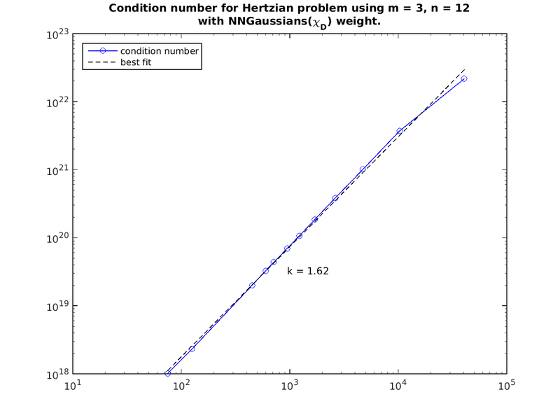
Herzian contact

The matrix of the Hertzian contact problem is shown below:

The condition number iz arther large and grows superlinearly with size in the example below.