Weighted Least Squares (WLS)
One of the most important building blocks of the meshless methods is the Moving Least Squares approximation, which is implemented in the EngineMLS class. Check EngineMLS unit tests for examples.
Basics
Our wish is to approximate an unknown function $u\colon \R^k \to \R$ while knowing $n$ values $u(x_i) := u_i$. The vector of known values will be denoted by $\b{u}$ and the vector of coordinates where those values were achieved by $\b{x}$. Note that $\b{x}$ is not a vector in the usual sense since its components $x_i$ are elements of $\R^k$, but we will call it vector anyway. The values of $\b{x}$ are called nodes or support nodes or support. The known values $\bf{u}$ are also called support values.
In general, an approximation function around point $p$ can be written as \[\hat{u} (p) = \sum_{i=1}^m \alpha_i b_i(p) = \b{b}(p)^\T \b{\alpha} \] where $\{b_i\}_{i=1}^m$ is a set of basis functions, and $\b{\alpha} = (\alpha_i)_{i=1}^m$ are the unknown coefficients.
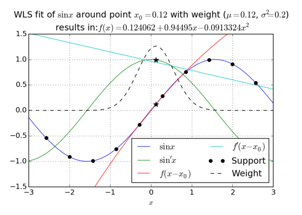
In MLS the goal is to minimize the error of approximation in given values, $\b{e} = \hat u(\b{x}) - \b{u}$ between the approximation function and target function in the known points $\b{x}$. Wee can choose to minimize any norm of the error vector $e$ and usually choose to minimize the 2-norm or square norm \[ \|\b{e}\| = \|\b{e}\|_2 = \sqrt{\sum_{i=1}^n e_i^2}. \] Commonly, we also choose to minimize a weighted norm instead \[ \|\b{e}\|_{2,w} = \|\b{e}\|_w = \sqrt{\sum_{i=1}^n (w_i e_i)^2}. \] The weights $w_i$ are assumed to be non negative and are assembled in a vector $\b{w}$ or a matrix $W = \operatorname{diag}(\b{w})$ and usually obtained from a weight function. A weight function is a nonnegative function $\omega\colon $
\[{r^2} = \sum\limits_j^n {W\left( {{{\mathbf{p}}_j}} \right){{\left( {u({{\mathbf{p}}_j}) - \hat u({{\mathbf{p}}_j})} \right)}^2}} = {\left( {{\mathbf{B\alpha }} - {\mathbf{u}}} \right)^{\text{T}}}{\mathbf{W}}\left( {{\mathbf{B\alpha }} - {\mathbf{u}}} \right)\]
Where $\b{B}$ is non-square matrix of dimension $m \times n$ and $\b{W}$ diagonal matrix of weights. The least squares problem can be solved with three approaches
- Normal equation (fastest - less accurate) - using Cholesky decomposition
- QR decomposition of $\b{B}$ ($rank(\b{B})=m$ - number of basis functions)
- SVD decomposition of $\b{B}$ (more expensive - more reliable, no rank demand)
In MM we use SVD.
Normal equations
We seek the minimum of \[{r^2} = {\left( {{\bf{u}} - {\bf{B\alpha }}} \right)^{\rm{T}}}\left( {{\bf{u}} - {\bf{B\alpha }}} \right)\] By seeking the zero gradient in terms of coefficient \[\frac{\partial }{{\partial {\alpha _i}}}\left( {{{\left( {{\bf{u}} - {\bf{B\alpha }}} \right)}^{\rm{T}}}\left( {{\bf{u}} - {\bf{B\alpha }}} \right)} \right) = 0\] resulting in \[{\bf{B}}{{\bf{B}}^{\rm{T}}}{\bf{\alpha }} = {{\bf{B}}^{\rm{T}}}{\bf{u}}\] The coefficient matrix $\bf{B}^T\bf{B}$ is symmetric and positive definite. However, solving above problem directly is poorly behaved with respect to round-off effects since the condition number of $\bf{B}^T\bf{B}$ is the square of that of $\bf{B}$. Or in case of weighted LS \[{\bf{WB}}{{\bf{B}}^{\rm{T}}}{\bf{\alpha }} = {\bf{W}}{{\bf{B}}^{\rm{T}}}{\bf{u}}\]
Complexity of Cholesky decomposition is $\frac{{{n}^{3}}}{3}$ and complexity of matrix multiplication $n{{m}^{2}}$
Pros: simple to implement, low computational complexity Cons: unstable
QR Decomposition
\[{\bf{B}} = {\bf{QR}} = \left[ {{{\bf{Q}}_1},{{\bf{Q}}_2}} \right]\left[ {\begin{array}{*{20}{c}} {{{\bf{R}}_1}}\\ 0 \end{array}} \right]\] \[{\bf{B}} = {{\bf{Q}}_1}{{\bf{R}}_1}\] $\bf{Q}$ is unitary matrix ($\bf{Q}^{-1}=\bf{Q}^T$). Useful property of a unitary matrices is that multiplying with them does not alter the (Euclidean) norm of a vector, i.e., \[\left\| {{\bf{Qx}}} \right\|{\bf{ = }}\left\| {\bf{x}} \right\|\] And $\bf{R}$ is upper diagonal matrix \[{\bf{R = (}}{{\bf{R}}_{\bf{1}}}{\bf{,}}0{\bf{)}}\] therefore we can say \[\begin{array}{l} \left\| {{\bf{B\alpha }} - {\bf{u}}} \right\| = \left\| {{{\bf{Q}}^{\rm{T}}}\left( {{\bf{B\alpha }} - {\bf{u}}} \right)} \right\| = \left\| {{{\bf{Q}}^{\rm{T}}}{\bf{B\alpha }} - {{\bf{Q}}^{\rm{T}}}{\bf{u}}} \right\|\\ = \left\| {{{\bf{Q}}^{\rm{T}}}\left( {{\bf{QR}}} \right){\bf{\alpha }} - {{\bf{Q}}^{\rm{T}}}{\bf{u}}} \right\| = \left\| {\left( {{{\bf{R}}_1},0} \right){\bf{\alpha }} - {{\left( {{{\bf{Q}}_1},{{\bf{Q}}_{\bf{2}}}} \right)}^{\rm{T}}}{\bf{u}}} \right\|\\ = \left\| {{{\bf{R}}_{\bf{1}}}{\bf{\alpha }} - {{\bf{Q}}_{\bf{1}}}{\bf{u}}} \right\| + \left\| {{\bf{Q}}_2^{\rm{T}}{\bf{u}}} \right\| \end{array}\] Of the two terms on the right we have no control over the second, and we can render the first one zero by solving \[{{\bf{R}}_{\bf{1}}}{\bf{\alpha }} = {\bf{Q}}_{_{\bf{1}}}^{\rm{T}}{\bf{u}}\] Which results in a minimum. We could also compute it with pseudo inverse \[\mathbf{\alpha }={{\mathbf{B}}^{-1}}\mathbf{u}\] Where pseudo inverse is simply \[{{\mathbf{B}}^{-1}}=\mathbf{R}_{\text{1}}^{\text{-1}}{{\mathbf{Q}}^{\text{T}}}\] (once again, R is upper diagonal matrix, and Q is unitary matrix). And for weighted case \[\mathbf{\alpha }={{\left( {{\mathbf{W}}^{0.5}}\mathbf{B} \right)}^{-1}}\left( {{\mathbf{W}}^{0.5}}\mathbf{u} \right)\]
Complexity of QR decomposition \[\frac{2}{3}m{{n}^{2}}+{{n}^{2}}+\frac{1}{3}n-2=O({{n}^{3}})\]
Pros: better stability in comparison with normal equations cons: higher complexity
SVD decomposition
In linear algebra, the singular value decomposition (SVD) is a factorization of a real or complex matrix. It has many useful applications in signal processing and statistics.
Formally, the singular value decomposition of an $m \times n$ real or complex matrix $\bf{B}$ is a factorization of the form $\bf{B}= \bf{U\Sigma V^\T}$, where $\bf{U}$ is an $m \times m$ real or complex unitary matrix, $\bf{\Sigma}$ is an $m \times n$ rectangular diagonal matrix with non-negative real numbers on the diagonal, and $\bf{V}^\T$ is an $n \times n$ real or complex unitary matrix. The diagonal entries $\Sigma_{ii}$ are known as the singular values of $\bf{B}$. The $m$ columns of $\bf{U}$ and the $n$ columns of $\bf{V}$ are called the left-singular vectors and right-singular vectors of $\bf{B}$, respectively.
The singular value decomposition and the eigen decomposition are closely related. Namely:
- The left-singular vectors of $\bf{B}$ are eigen vectors of $\bf{BB}^\T$.
- The right-singular vectors of $\bf{B}$ are eigen vectors of $\bf{B}^\T{B}$.
- The non-zero singular values of $\bf{B}$ (found on the diagonal entries of $\bf{\Sigma}$) are the square roots of the non-zero eigenvalues of both $\bf{B}^\T\bf{B}$ and $\bf{B}^\T \bf{B}$.
with SVD we can write \bf{B} as \[\bf{B}=\bf{U\Sigma{{V}^{\T}}}\] where are \bf{U} and \bf{V} again unitary matrices and $\bf{\Sigma}$ stands for diagonal matrix of singular values.
Again we can solve either the system or compute pseudo inverse as
\[ \bf{B}^{-1} = \left( \bf{U\Sigma V}^\T\right)^{-1} = \bf{V}\bf{\Sigma^{-1}U}^\T \] where $\bf{\Sigma}^{-1}$ is trivial, just replace every non-zero diagonal entry by its reciprocal and transpose the resulting matrix. The stability gain is exactly here, one can now set threshold below which the singular value is considered as 0, basically truncate all singular values below some value and thus stabilize the inverse.
SVD decomposition complexity \[ 2mn^2+2n^3 = O(n^3) \]
Pros: stable cons: high complexity
