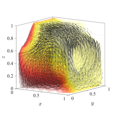
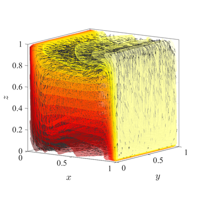
Natural convection in 3D irregular domain

The classical De Vahl Davis natural convection test can be extended to 3D. In below figures steady state temperature contour and velocity quiver plots for Ra$=10^6$ case in 3D are presented. A more quantitative analysis is done by comparing characteristic values, i.e.\ peak positions and values of cross section velocities, with data available in literature~\cite{couturier2000performance, kosec2008solution, wang2017numerical, fusegi1991numerical}. We analyze six different cases, namely $\textup{Ra} = 10^6,10^7,10^8$ in 2D, and $\textup{Ra} = 10^4,10^5,10^6$ in 3D. The comparison in presented in~\cref{tab:ff-data}.

All spatial operators are discretized using RBF-FD with $r^3$ PHS radial basis functions, augmented with monomials up to order $2$, with the closest $25$ nodes used as a stencil. For the time discretization time step $\Delta t=10^{-3}$ was used for all cases. Nodal distance $h=0.01$ is used for simulations in 2D and $h=0.25$ for simulations in 3D. Boundaries with Neumann boundary conditions are additionally treated with ghost nodes Ghost nodes (theory).

\begin{table}[h] \centering \caption{Comparison of results computed with RBF-FD on FF nodes and reference data. } \label{tab:ff-data} \renewcommand{\arraystretch}{1.2} \scalebox{0.68}{ \begin{tabular}{|l|l|l|l|l|l|l|l|l|l|l|l|l|l|} \cline{2-14} \multicolumn{1}{c|}{} & \multirow{2}{*}{\textbf{Ra}} & \multicolumn{3}{c|}{$v_{max}(x, 0.5)'"`UNIQ-MathJax11-QINU`"'x'"`UNIQ-MathJax12-QINU`"'u_{max}(0.5, y)'"`UNIQ-MathJax13-QINU`"'y'"`UNIQ-MathJax14-QINU`"'10^6'"`UNIQ-MathJax15-QINU`"'10^7'"`UNIQ-MathJax16-QINU`"'10^8'"`UNIQ-MathJax17-QINU`"'w_{max}(x, 0.5,0.5)'"`UNIQ-MathJax18-QINU`"'x'"`UNIQ-MathJax19-QINU`"'u_{max}(0.5, 0.5, z)'"`UNIQ-MathJax20-QINU`"'z'"`UNIQ-MathJax21-QINU`"'10^4'"`UNIQ-MathJax22-QINU`"'10^5'"`UNIQ-MathJax23-QINU`"'10^6$ & 0.2564 & 0.2556 & 0.2588 & 0.961 & 0.965 & 0.966 & 0.0841 & 0.0816 & 0.0841 & 0.143 & 0.140 & 0.144 \\ \hline \end{tabular}

 }

\end{table}