Meshless Local Strong Form Method (MLSM)
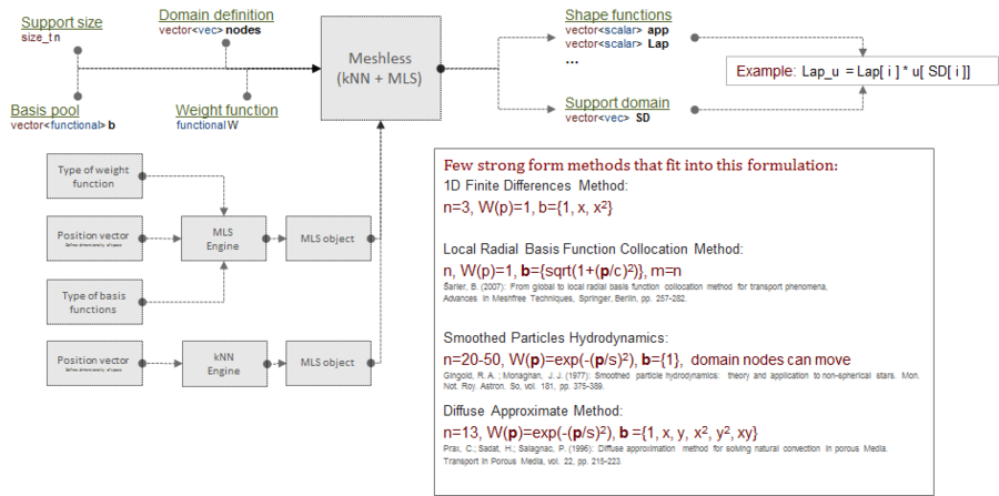
The Meshless Local Strong Form Method (MLSM) is a generalization of methods which are in literature also known as Diffuse Approximate Method (DAM), Local Radial Basis Function Collocation Methods (LRBFCM), Generalized FDM, Collocated discrete least squares (CDLS) meshless, etc. Although each of the named methods pose some unique properties, the basic concept of all local strong form methods is similar, namely to approximate treated fields with nodal trial functions over the local support domain. The nodal trial function is then used to evaluate various operators, e.g. derivation, integration, and after all, approximation of a considered field in arbitrary position. The MLSM could easily be understood as a meshless generalization of the FDM, however much more powerful. MLSM has an ambition to avoid using pre-defined relations between nodes and shift this task into the solution procedure. The final goal of such an approach is higher flexibility in complex domains.
The elegance of MLSM is its simplicity and generality. The presented methodology can be also easily upgraded or altered, e.g. with nodal adaptation, basis augmentation, conditioning of the approximation, etc., to treat anomalies such as sharp discontinues or other obscure situations, which might occur in complex simulations. In the MLSM, the type of approximation, the size of support domain, and the type and number of basis function is general. For example minimal support size for 2D transport problem (system of PDEs of second order) is five, however higher support domains can be used to stabilize computations on scattered nodes at the cost of computational complexity. Various types of basis functions might appear in the calculation of the trial function, however, the most commonly used are multiquadrics, Gaussians and monomials. Some authors also enrich the radial basis with monomials to improve performance of the method. All these features can be controlled on the fly during the simulation. From the computation point of view, the localization of the method reduces inter-processor communication, which is often a bottleneck of parallel algorithms.
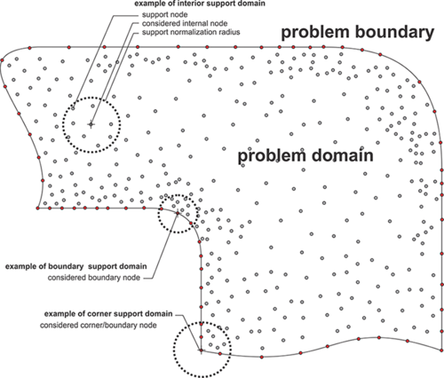
The core of the spatial discretization is a local Moving Least Squares (MLS) approximation of a considered field over the overlapping local support domains, i.e. in each node we use approximation over a small local sub-set of neighbouring $n$ nodes. The trial function is thus introduced as \[\hat{u}(\mathbf{p})=\sum\limits_{i}^{m}{{{\alpha }_{i}}{{b}_{i}}(\mathbf{p})}=\mathbf{b}{{\left( \mathbf{p} \right)}^{\text{T}}}\mathbf{\alpha }\] with $m,\,\,\mathbf{\alpha }\text{,}\,\,\mathbf{b},\,\,\mathbf{p}\left( {{p}_{x}},{{p}_{y}} \right)$ standing for the number of basis functions, approximation coefficients, basis functions and the position vector, respectively.
The problem can be written in matrix form (refer to Moving Least Squares (MLS) for more details) as \[~\mathbf{\alpha }={{\left( {{\mathbf{W}}^{0.5}}\mathbf{B} \right)}^{+}}{{\mathbf{W}}^{0.5}}\mathbf{u}\] where $(\mathbf{W}^{0.5}\mathbf{B})^{+}$ stand for a Moore–Penrose pseudo inverse.
Shape functions
By explicit expressiong the coefficients $\alpha$ into the trial function \[~\hat{u}\left( \mathbf{p} \right)=\mathbf{b}{{\left( \mathbf{p} \right)}^{\text{T}}}{{\left( {{\mathbf{W}}^{0.5}}\left( \mathbf{p} \right)\mathbf{B} \right)}^{+}}{{\mathbf{W}}^{0.5}}\left( \mathbf{p} \right)\mathbf{u}=\mathbf{\chi }\left( \mathbf{p} \right)\mathbf{u}\] is obtained, where $\mathbf{\chi}$ stand for the shape functions. Now, we can apply partial differential operator, which is our goal, on the trial function \[L~\hat{u}\left( \mathbf{p} \right)=L\mathbf{\chi }\left( \mathbf{p} \right)\mathbf{u}\] where L stands for general differential operator. For example: \[{{\mathbf{\chi }}^{\partial x}}\left( \mathbf{p} \right)=\frac{\partial }{\partial x}~\mathbf{b}{{\left( \mathbf{p} \right)}^{\text{T}}}{{\left( {{\mathbf{W}}^{0.5}}\left( \mathbf{p} \right)\mathbf{B} \right)}^{+}}{{\mathbf{W}}^{0.5}}\] \[{{\mathbf{\chi }}^{\partial y}}\left( \mathbf{p} \right)=\frac{\partial }{\partial y}~\mathbf{b}{{\left( \mathbf{p} \right)}^{\text{T}}}{{\left( {{\mathbf{W}}^{0.5}}\left( \mathbf{p} \right)\mathbf{B} \right)}^{+}}{{\mathbf{W}}^{0.5}}\] \[{{\mathbf{\chi }}^{{{\nabla }^{2}}}}\left( \mathbf{p} \right)={{\nabla }^{2}}\mathbf{b}{{\left( \mathbf{p} \right)}^{\text{T}}}{{\left( {{\mathbf{W}}^{0.5}}\left( \mathbf{p} \right)\mathbf{B} \right)}^{+}}{{\mathbf{W}}^{0.5}}\]
The presented formulation is convenient for implementation since most of the complex operations, i.e. finding support nodes and building shape functions, are performed only when nodal topology changes. In the main simulation, the pre-computed shape functions are then convoluted with the vector of field values in the support to evaluate the desired operator. The presented approach is even easier to handle than the FDM, however, despite its simplicity it offers many possibilities for treating challenging cases, e.g. nodal adaptivity to address regions with sharp discontinuities or p-adaptivity to treat obscure anomalies in physical field, furthermore, the stability versus computation complexity and accuracy can be regulated simply by changing number of support nodes, etc. All these features can be controlled on the fly during the simulation by re computing the shape functions with different setups. However, such re-setup is expensive, since the \[\mathbf{b}{{\left( \mathbf{p} \right)}^{\text{T}}}{{\left( {{\mathbf{W}}^{0.5}}\left( \mathbf{p} \right)\mathbf{B} \right)}^{+}}{{\mathbf{W}}^{0.5}}\] has to be re-evaluated, with asymptotical complexity of $O\left( {{N}_{D}}n{{m}^{2}} \right)$, where ${{N}_{D}}$ stands for total number of discretization nodes. In addition, the determination of support domain nodes also consumes some time, for example, if a kD-tree [20] data structure is used, first the tree is built with $O\left( {{N}_{D}}\log {{N}_{D}} \right)$ and then additional $O\left( {{N}_{D}}\left( log{{N}_{D}}+n \right) \right)$ for collecting n supporting nodes.
References
- Kosec G., A local numerical solution of a fluid-flow problem on an irregular domain. Advances in engineering software. 2016;7 ; [29512743] :: manuscript
- Trobec R., Kosec G., Šterk M., Šarler B., Comparison of local weak and strong form meshless methods for 2-D diffusion equation. Engineering analysis with boundary elements. 2012;36:310-321; manuscript
- Kosec G, Sarler B. Solution of thermo-fluid problems by collocation with local pressure correction. International Journal of Numerical Methods for Heat & Fluid Flow. 2008;18:868-82 manuscript
- Trobec R., Kosec G., Parallel Scientific Computing, ISBN: 978-3-319-17072-5 (Print) 978-3-319-17073-2.

