Burgers' equation

Let us consider the Burgers' equation, which describes the dynamics of viscous fluid without the effects of pressure. Despite being unrealistic, it is the simplest description of advective flow with diffusive effects of viscosity. It has the following form: \begin{equation} \frac{\partial \b{u}}{\partial t} + (\b{u}\cdot\nabla)\b{u} = \nu \nabla^2 \b{u} , \end{equation}

where $\b{u}$ is a velocity field. For time stepping the advection term must be linearized. There are several tactics of linearization, but we choose the simplest one, which is using the previous velocity as an approximantion of the current velociy. Using the implicit Euler method we arrive at the equation

\begin{equation} \b{u}^{n}_i + \Bigl[\b{u}^{n-1}_i\cdot\nabla_i\b{u}^{n} - \nu\nabla^2_i \b{u}^{n}\Bigr]\Delta t = \b{u}^{n-1}_i, \end{equation}

where the subscript $i$ is the index of the domain node, superscripts $n$ and $n-1$ denote the current and the previous time step respectively, $\Delta t$ is the length of the time step. The notation $\nabla_i$ means the gradient operator at node $i$, not the component of the gradient. Same holds for $\nabla^2_i$. Using the Medusa library, this equation can be solved for $\b{u}^{n}_i$.

Solution in 1D

Let's look at an example in 1D with Dirichlet boundary conditions. We are solving the equivalent of equation (2) but with only one spatial variable: \begin{equation} u^{n}_i + \Bigl[u^{n-1}_i\frac{\partial u^{n}}{\partial x} - \nu\frac{\partial^2 u^{n}}{\partial x^2}\Bigr]\Delta t = u^{n-1}_i ,\\ u_i = 0 \text{ on } \partial \Omega . \end{equation}

This will be rewritten into a linear system of equations with Medusa and then solved with Eigen. Let's look at the code(find the full version in our repository).

1 // Build 1D domain
2 BoxShape<Vec1d> domain((-l), (l)); // the interval [-l, l]
3 auto discretization = domain.discretizeWithStep(dx);
4 int domain_size = discretization.size();
5 // Find support nodes
6 FindClosest find_support(5);
7 discretization.findSupport(find_support);

First we construct our 1D domain with lenght 2l, discretize it with a given step dx and find the closest 5 nodes of each node which are called stencil nodes.

1 Polyharmonic<double, 3> p;
2 Monomials<Vec1d> mon(4);
3 RBFFD<Polyharmonic<double, 3>, Vec1d, ScaleToClosest>
4         approx(p, mon);
5 auto storage = discretization.computeShapes(approx); 
6 VectorXd E1 = VectorXd::Zero(domain_size);  // vector for containing the current state

We will use polyharmonic splines of order 3 as Radial Basis Functions(RBFs) augmented with monomials up to 4th order for our approximation engine. We use it in conjunction with stencil nodes to compute the stencil weights(also called shape functions) which are used in approximations of differential operators on our domain. Next we set the initial condition to $$u(x, 0) = \frac{2\nu ake^{-\nu k^2t}\sin(kx)}{b + ae^{-\nu k^2t}\cos(kx)},$$ where $a, b, k$ are constants. We chose this function because it has an analytical solution which we will compare our solution to. It is derived using the Cole-Hopf transformation of a solution of the diffusion equation with the initial profile $f(x) = b + a\cos(kx)$ for $b>a$.

1     //Set initial condition 
2     for (int i : discretization.all()){ 
3         E1(i) = 2*visc*a*k*std::exp(-visc*pow(k,2)*t_0)*std::sin(k*discretization.pos(i,0))/(b+a*std::exp(- 
4         visc*pow(k,2)*t_0)*std::cos(k*discretization.pos(i,0)));

Inside our time-stepping loop, we instantiate the matrix $M$ and the vector $rhs$ representing the linear system. We then construct the differential operators for implicit solving.

1 for (tt = 1; tt <= t_steps; ++tt) {
2     SparseMatrix<double> M(domain_size, domain_size); // construct matrix of apropreate size
3     VectorXd rhs = VectorXd::Zero(domain_size); 
4     M.reserve(Range<int>(domain_size, n));
5     auto op = storage.implicitOperators(M, rhs);  // compute the implicit operators

Now comes the crucial part - setting the equation. In essence, we rewrite equation (3) in Medusa's terms. Terms on the left hand side are written into matrix $M$ and the terms on the right into $rhs$. The terms with the prefix op. are matrices that represent the appropriate differential operators(op.value(i) is a matrix with $A_{ii}$ = 1 and zero everywhere else), vector E1[i] represents $\b{u}_i^{n-1}$ - result of the previous step.

1     // Setting the equation 
2     for (int i : interior) {
3         op.value(i) + (E1[i] * dt) * op.der1(i, 0) + (-dt*visc) * op.der2(i, 0, 0) = E1[i];  
4 }

Boundary conditions are handled in the same way. Here we set Dirichlet boundary conditions.

1     // Setting Dirichlet boundary conditions
2     for (int i : boundary) {
3         op.value(i) = 0;  
4 }

We then solve the equation and update E1 for use in the next time step. The solution is also saved into an output file with HDF5.

 1     M.makeCompressed(); // Optimization
 2     BiCGSTAB<SparseMatrix<double, RowMajor>> solver; // Creating solver object
 3     solver.compute(M); // Initialize the iterative solver
 4 
 5     // Solve the linear system and update the state
 6     VectorXd E2 = solver.solve(rhs);
 7     E1 = E2;
 8 
 9     if (tt%(t_factor) == 0) {
10         // Saving state in output file
11         hdf_out.openGroup("/step" + std::to_string(t_save));
12         hdf_out.writeSparseMatrix("M", M);
13         hdf_out.writeDoubleAttribute("TimeStep", t_save);
14         std::cout<< "Time step " << t_save << " of " << t_steps/t_factor << "." << std::endl;
15         hdf_out.writeDoubleAttribute("time",(t_0 + tt * dt));
16         ++t_save;
17         hdf_out.writeDoubleArray("E", E1);
18         }

Results

For our simulation we used the following parameters: \begin{align*} \nu &= 1,\\ l &= 1,\\ a &= 4,\\ b &= 4,\\ k &= \frac{4\pi}{2l},\\ \phi(r) &= r^3,\\ n &= 5,\\ m &= 4. \end{align*} As mentioned before the support of each node are its 5 closest nodes including the node itself. We used the RBF-FD method with polyharmonic splines of order 3 augmented with polynomials of up to order 4. Animation of the result is shown below.

Convergence

Spatial discretization

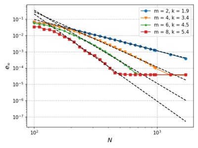
We use the RBF-FD method with PHS radial basis function $\phi(r) = r^3$ and fix the time step to $dt = 10^{-6}$. We vary the polynomial augmentation order $m \in \{2, 4, 6, 8\}$ and analize the convergence with increasing number of discretization nodes N.

After some initial oscilation the error decreases as $O(h^k)$, where $k$ is the fit parameter for every $m$ and $h$ is the distance between consecutive nodes. But eventualy it becomes constant value. The reason is that for finer spatial discretizations we are bounded by the time step because of linearization.

Temporal discretization

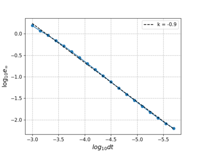
Now we fix $N$ and $m$ to 1024 and 4 and vary the size of the time step from $10^{-3}$ to $10^{-6}$. The error decreases linearly with the time step.

Solution in 2D

In 2D the Burgers' equation (1) gives a system of two coupled nonlinear equations: \begin{gather} \frac{\partial u}{\partial t} + u\frac{\partial u}{\partial x} + v\frac{\partial u}{\partial y} = \nu\nabla^2u,\\ \frac{\partial v}{\partial t} + u\frac{\partial v}{\partial x} + v\frac{\partial v}{\partial y} = \nu\nabla^2v, \end{gather} where $u$ and $v$ are ve;ocities in the $x$ and $y$ direction respectively. We discretize equations (4) and (5) in the same way as in the 1D case: \begin{gather} u^{n}_i + \Bigl[u^{n-1}_i\frac{\partial u^{n}}{\partial x} + v^{n-1}_i\frac{\partial u^{n}}{\partial y} - \nu\nabla^2u^{n}\Bigr]\Delta t = u^{n-1}_i ,\\ v^{n}_i + \Bigl[u^{n-1}_i\frac{\partial v^{n}}{\partial x} + v^{n-1}_i\frac{\partial v^{n}}{\partial y} - \nu\nabla^2v^{n}\Bigr]\Delta t = v^{n-1}_i . \end{gather} We will solve each equation separately every time step, this will enable us to partialy parallelize the algorithm. First we contruct a 2D square domain with side length of 1 and find n closest nodes of each node.

1 BoxShape<Vec2d> b((0, 0), (a, a));
2 double step = std::stod(argv[1]);
3 auto discretization = b.discretizeBoundaryWithStep(step);
4 GeneralFill<Vec2d> fill; fill.seed(0);
5 discretization.fill(fill, step);
6 Find support nodes
7 discretization.findSupport(FindClosest(n));
8 int domain_size = discretization.size();

We will be simulating the following initial and boundary conditions: \begin{gather*} u(x,y,0) = sin(\pi x)cos(\pi y),\\ v(x,y,0) = cos(\pi x)sin(\pi y),\\ u(0,y,t)=u(1,y,t)=v(x,0,t)=v(x,1,t)=0. \end{gather*} The analytical solution is given here . In the time stepping loop we use #pragma omp parallel sections to enable concurrent solving for $u$ and $v$. In each section we define separate matricies Mu or Mv, rhs vectors rhu and rhv, and implicit operators opu and opv which will write into their respective matricies. The code bellow includes only the section for $u$. The types -1 ,-2 , -3 ,-4 correspond to the left, right, bottom and top boundaries. At the end of each section the velocities are updated.

 1 for (tt = 1; tt <= t_steps; ++tt) {
 2 
 3 double t = t_0 + tt * dt;
 4 
 5 #pragma omp parallel sections shared(domain_size, discretization, storage, dt, u, v) 
 6 {
 7     ////Solving for u////
 8     #pragma omp section
 9     {
10         SparseMatrix<double, RowMajor> Mu(domain_size, domain_size); // construct matrix of apropreate size
11         VectorXd rhu = VectorXd::Zero(domain_size);  // set empty vector for rhs
12         auto opu = storage.implicitOperators(Mu, rhu);        
13         Mu.reserve(storage.supportSizes());
14 
15         // Setting the equation 
16         #pragma omp parallel for
17         for (int i : discretization.interior()) {
18             opu.value(i) + (u[i]*dt) * opu.der1(i, 0) + (v[i]*dt) * opu.der1(i, 1) + (-1/rndls*dt) * opu.lap(i) = u[i];  
19         }
20         // Boundary conditions
21         for (int i : discretization.types() == -3){
22             opu.value(i) = analytical_u(discretization.pos(i,0), discretization.pos(i,1), t, 1.0/rndls);
23         }
24         for (int i : discretization.types() == -4){
25             opu.value(i) = analytical_u(discretization.pos(i,0), discretization.pos(i,1), t, 1.0/rndls);
26         }
27         for (int i : discretization.types() == -1){
28             opu.value(i) = 0.0;
29         }
30         for (int i : discretization.types() == -2){
31             opu.value(i) = 0.0;
32         }
33         Mu.makeCompressed(); 
34         BiCGSTAB<SparseMatrix<double, RowMajor>> solveru; // Creating solver object
35         solveru.compute(Mu); // Initialize the iterative solver
36         VectorXd u2 = solveru.solve(rhu);
37         u = u2;
38     }

References

- ↑ Q. Gao, M.Y. Zou, An analytical solution for two and three dimensional nonlinear Burgers' equation, Applied Mathematical Modelling, Volume 45, 2017, Pages 255-270, ISSN 0307-904X, https://doi.org/10.1016/j.apm.2016.12.018.