HP-adaptivity

edit 

Related papers

M. Jančič, G. Kosec; Strong form mesh‑free hp‑adaptive solution of linear elasticity problem, Engineering with computers, vol. 39, 2023 [DOI: 10.1007/s00366-023-01843-6]

Adaptive solution procedures are essential in problems where the accuracy of the numerical solution varies spatially and are currently subject of intensive studies. Two conceptually different adaptive approaches have been proposed, namely $p$-adaptivity or $h$-, $r$-adaptivity. In $p$-adaptivity, the accuracy of the numerical solution is varied by changing the order of approximation, while in $h$- and $r$-adaptivity the resolution of the spatial discretization is adjusted for the same purpose. In the $h$-adaptive approach, nodes are added or removed from the domain as needed, while in the $r$-adaptive approach, the total number of nodes remains constant - the nodes are only repositioned with respect to the desired accuracy. Ultimately, $h$- and $p$-adaptivities can be combined to form the so-called $hp$-adaptivity, where the accuracy of the solution is controlled with the order of the method and the resolution of the spatial discretization.

Basic concept

The proposed $hp$-adaptive solution procedure follows the well-established paradigm based on an iterative loop, where each iteration step consists of four modules:

• Solve - A numerical solution $\widehat{u}$ is obtained.
• Estimate - An estimate of the spatial accuracy of the numerical solution is calculated using error indicators.
• Mark - Depending on the error indicator values $\eta _i$, a marking strategy is used to mark the computational nodes for (de)refinement.
• Refine - Refinement strategy is employed to define the amount of the (de)refinement.

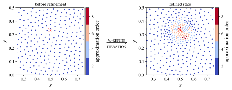
Expected result is drafted in figure below.

Implementation

The implementation of $hp$-adaptive solution procedure can be found here.

Solution procedure

Solve

First a numerical solution $\widehat{u}$ to the governing problem must be obtained. In general, the numerical treatment of a system of PDEs is done in several steps. First, the domain is discretized by positioning the nodes, then the linear differential operators in each computational node are approximated, and, finally, the system of PDEs is discretized and assembled into a large sparse linear system. To obtain a numerical solution $\widehat{u}$, the sparse system is solved.

Estimate (IMEX error indicator)

In the estimation step, critical areas with high error of the numerical solution are identified. Identifying such areas is not a trivial task. In rare cases, where a closed form solution to the governing system of PDEs exists, we can not only indicate such areas but also estimate the accuracy of the numerical solution. However, for real-world problems, which are often subject of numerical simulations, closed form solutions do not exist. Therefore, other objective metrics are needed to indicate the computational nodes with high error of the numerical solution. Numerical tools used in such cases are commonly referred to as error indicators.

We have chosen to use our own error indication algorithm IMEX for implementation-related convenience reasons. This error indicator makes use of the implicitly obtained numerical solution and explicit operators (approximated by higher-order basis) to reconstruct the right-hand side of the governing problem.

To further explain basic idea of IMEX, let us define a PDE of type: $$ \mathcal L u = f_{RHS}, $$ where $\mathcal L$ is a differential operator applied to the scalar field $u$ and $f_{RHS}$ is a function. To obtain an error indicator field $\eta$, the problem is first solved implicitly by using a lower order approximation of operators $\mathcal L$, $\mathcal L^{(lo)}_{im}$, obtaining the solution $u^{(im)}$ in the process. The implicitly computed field $u^{(im)}$ is then used to explicitly reconstruct the right-hand side of the governing problem, but this time using a higher order approximation of $\mathcal L$, $\mathcal L^{(hi)}_{ex}$, obtaining $f_{RHS}^{(ex)}$ in the process. Finally, $f_{RHS}^{(ex)}$ and $f_{RHS}$ are compared $\eta = \left | f_{RHS} - f_{RHS}^{(ex)} \right |$ to indicate the error of the numerical solution.

Mark

After the error indicator $\eta$ had been obtained for each computational point in $\Omega$, a marking strategy is employed. The main objective of this step is to flag the nodes with too high or too low error indicator values in order to achieve a uniformly distributed precision of the numerical solution and reduce computational costs - by avoiding fine local field descriptions and high order approximations where this is not required. Furthermore, the marking strategy not only decides whether or not (de)refinement should take place at a given computational node, but also defines the type of the refinement procedure in cases where there are multiple to choose from.

In each adaptivity iteration, the marking strategy starts by checking the error indicator values $\eta _i$ for all computational nodes in the domain. If $\eta _i$ is greater than $\alpha \eta_{max}$ for a free model parameter $\alpha \in (0, 1)$, the node is marked for refinement. If $\eta _i$ is less than $\beta \eta_{max}$ for a free model parameter $\beta \in (0,1) \land \beta \leq \alpha$, the node is marked for derefinement. Otherwise, the node is left unmarked meaning no refinement should take place. The marking strategy can be summarized with a single equation $$ \begin{cases} \eta _i > \alpha \eta_{max}, & \text{ refine} \\ \beta \eta_{max} \leq \eta _i \leq \alpha \eta_{max}, & \text{ do nothing} \\ \eta _i < \beta \eta_{max}, & \text{ derefine} \end{cases}. $$

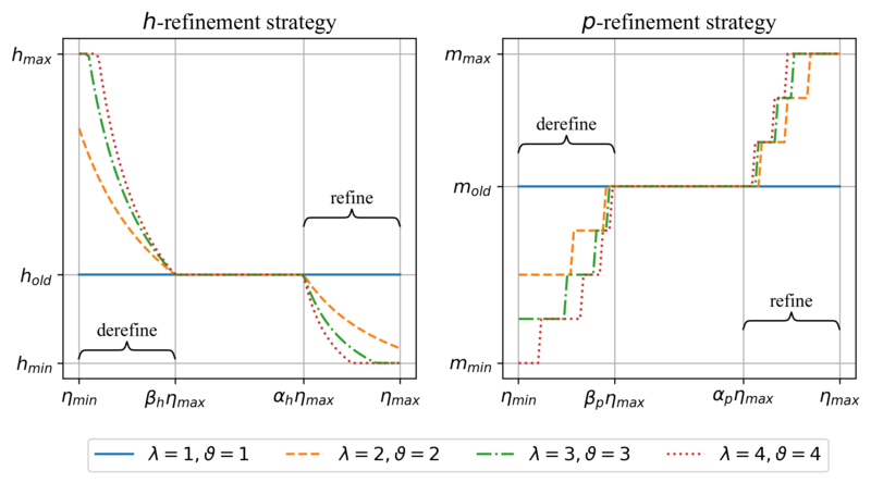
In the context of mesh-based methods, it has already been observed, that this strategy is indeed simple to implement, however, far from optimal in terms of achieving good convergence rates. Our studies have shown that a slight modification to the originally proposed strategy can significantly improve the performance of an $hp$-adaptive solution procedure in the context of mesh-free methods, but at the cost of higher number of free parameters - making it more difficult to understand. Nevertheless, the strategy is modified by introducing parameters $\left \{ \alpha_h, \beta_h \right \}$ and $\left \{ \alpha_p, \beta_p \right \}$ for separate treatment of $h$- and $p$-refinements respectively. A schematic is shown in figure below.

Refine

After obtaining the list of nodes marked for modification, the refinement module is initialized. In this module, the local field description and local approximation order for the unmarked nodes are left unchanged, while the rest are further processed to determine other refinement-type-specific details - such as the amount of the (de)refinement.

We use the following $h$-refinement rule $$ \label{eq:refinement} h_i^{new}(\b p) = \frac{h_i^{old}}{\frac{\eta_i - \alpha \eta _{max}}{\eta_{max} - \alpha\eta_{max}}\big(\lambda - 1\big) + 1} $$ for the dimensionless parameter $\lambda \in [1, \infty)$ allowing us to control the aggressiveness of the refinement - the larger the value, the greater the change. This refinement rule also conveniently refines the areas with higher error indicator values more than the ones that are closer to the upper refinement threshold $\alpha_h \eta_{max}$. Similarly, a derefinement rule is proposed $$ \label{eq:derefinement} h_i^{new}(\b p) = \frac{h_i^{old}}{\frac{\beta \eta _{max} - \eta_i}{\beta\eta_{max} - \eta_{min}}\big(\frac{1}{\vartheta} - 1\big) + 1}, $$ where parameter $\vartheta \in [1, \infty)$ allows us to control the aggressiveness of derefinement.

The same refinement and derefinement strategies were applied to control the local approximation order, except this time the value is rounded to the nearest integer. Similarly and for the same reasons as we did with the marking strategy, we consider a separate treatment of $h$- and $p$-adaptive procedures, by introducing (de)refinement aggressiveness parameters $\left \{\lambda_h, \vartheta_h \right \}$ and $\left \{\lambda_p, \vartheta_p \right \}$ for $h$- and $p$-refinement types respectively.

Finalization step

Before the 4 modules can be iteratively repeated, the domain is rediscretized taking into account the newly computed local internodal distances $h_i^{new}(\b p)$ and the local approximation orders $m_i^{new}(\b p)$. However, both are only known in the computational nodes, while global functions $\widehat{h}^{new}(\b p)$ and $\widehat{m}^{new}(\b p)$ over our entire domain space $\Omega$ are required. These are obtained by employing the Sheppard's inverse distance weighting interpolation.

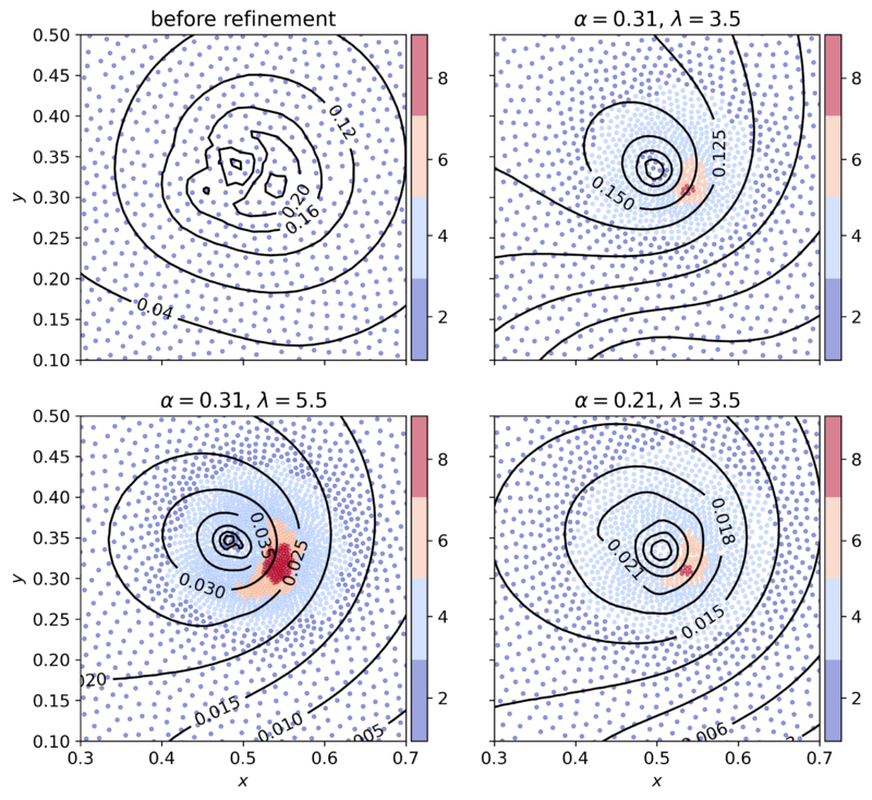
Figure below schematically demonstrates 3 examples of $hp$-refinements. For the sake of demonstration, the refinement parameters for $h$- and $p$-adaptivity are the same, i.e. $\left \{ \alpha, \beta, \lambda, \vartheta \right \} = \left \{ \alpha_h, \beta_h, \lambda_h, \vartheta_h \right \} = \left \{ \alpha_p, \beta_p, \lambda_p, \vartheta_p \right \}$. Additionally, the derefinement aggressiveness $\vartheta$ and the upper threshold $\beta$ are kept constant, so, effectively, only the upper bound of refinement $\alpha$ and refinement aggressiveness $\lambda$ are altered. We observe that the effect refinement parameters is somewhat intuitive. The larger the aggressiveness $\lambda$ the better the local field description and the larger the number of nodes with high approximation order. Similar effect is observed with manipulating the upper refinement threshold $\alpha$, except the effect comes at a smoother manner. Also observe that all refined states were able to increase the accuracy of the numerical solution from the initial state.

Examples

Example peak problem

The proposed $hp$-adaptive solution procedure is demonstrated on a synthetical example. We chose a 2-dimensional Poisson problem with exponentially strong source positioned at $\boldsymbol x_s = \Big (\frac{1}{2}, \frac{1}{3}\Big )$. This example is categorized as a difficult problem and is commonly used to test the performance of adaptive solution procedures. The problem has a tractable solution $u(\boldsymbol x)=e^{-a \left \| \boldsymbol x - \boldsymbol x_s \right \|^2}$, which allows us to evaluate the precision of the numerical solution $\widehat{u}$, e.g.\ in terms of the infinity norm.

Governing equations are $$ \nabla^2 u (\boldsymbol x) = 2a e^{-a \left \| \boldsymbol x - \boldsymbol x_s \right \|^2}(2a\left \| \boldsymbol x - \boldsymbol x_s \right \| - d) \quad \quad \text{in } \Omega, \\ u (\boldsymbol x) = e^{-a \left \| \boldsymbol x - \boldsymbol x_s \right \|^2} \quad \quad \text{on } \Gamma_d, \\ \nabla u (\boldsymbol x) = -2a(\boldsymbol x - \boldsymbol x_s)e^{-a \left \| \boldsymbol x - \boldsymbol x_s \right \|^2} \quad \quad\text{on } \Gamma_n, $$

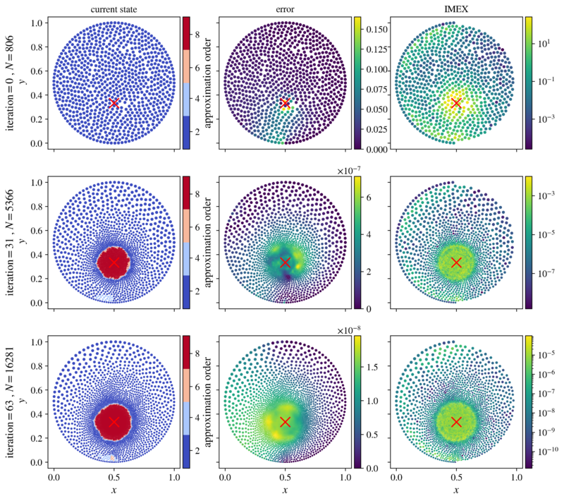
Figure below shows example indicator fields for initial iteration, intermediate iteration and iteration that achieved the best accuracy of the numerical solution. The third column shows the IMEX error indicator. We can see that the IMEX successfully located the position of the strong source at $\boldsymbol x_s = \Big (\frac{1}{2}, \frac{1}{3}\Big )$ as the highest indicator values are seen in its neighborhood. Moreover, the second column shows that the accuracy of the numerical solution and uniformity of error distribution have both been significantly improved by the $hp$-adaptive solution procedure, further proving that the IMEX can be successfully employed as a reliable error indicator.

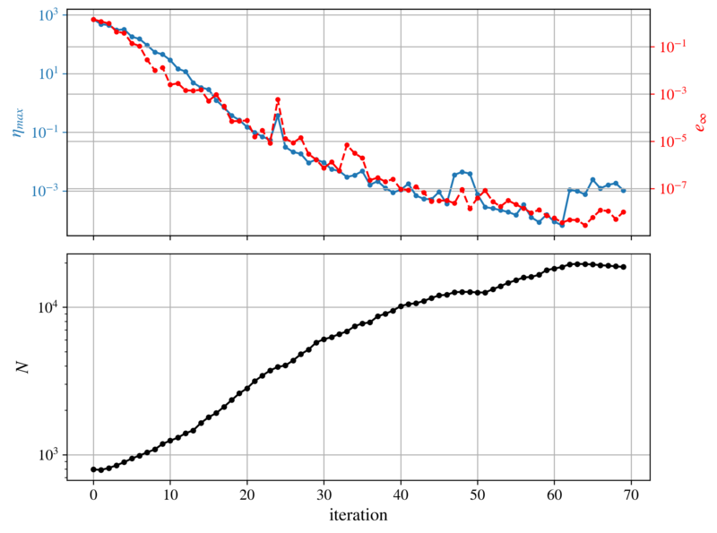
The behavior of IMEX over 70 adaptivity iterations is further studied in figure below. We are pleased to see that the convergence limit of the indicator around iteration $N_{iter}=60$ agrees well with the convergence limit of the numerical solution.

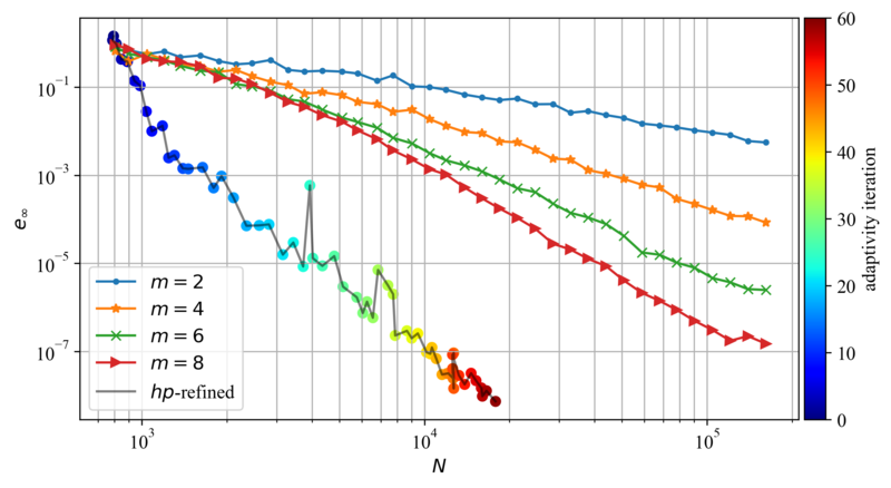
Finally, the convergence behavior of the proposed $hp$-adaptive solution procedure is studied. In addition to the convergence of a single $hp$-adaptive run, the convergences obtained without the use of refinement procedures, i.e. solutions obtained with uniform internodal spacing and approximation orders over the entire domain, are shown in figure below. The figure evidently shows that a $hp$-adaptive solution procedure was able to notably improve the numerical solution in terms of accuracy and required computational points.

Application to linear elasticity problems: Fretting fatigue contact

The application of the proposed $hp$-adaptive solution procedure is further expanded to study a linear elasticity problem. Specifically, we obtain a $hp$-refined solution to fretting fatigue contact problem , for which the authors believe no closed form solution is known.

The problem formulation is given here .

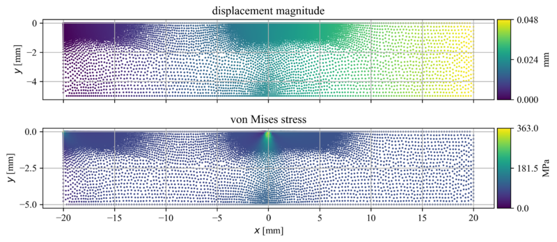
Figure below shows an example of $hp$-refined solution to fretting fatigue problem at the last adaptivity iteration with $N=46\,626$ computational nodes. We see that the solution procedure successfully located the two critical points, i.e. the fixed top left corner with a stress singularity and the area in the middle of the top edge where the contact is simulated. Note that the highest stress values (approximately $2$ times higher) have been computed in the singularity in the top left corner, but those nodes are not shown since our focus is shifted towards the area under the contact.

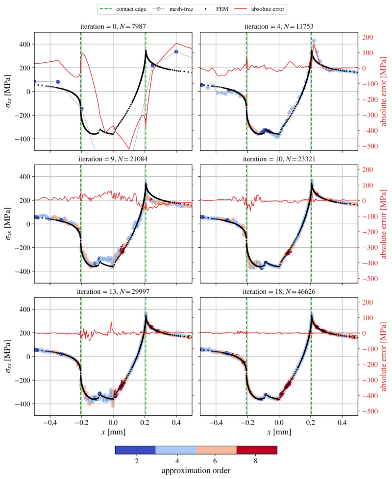
For a detailed analysis, we look at the surface traction $\sigma_{xx}$, as it is often used to determine the location of crack initiation. The surface traction is shown in figure below for $6$ selected adaptivity iterations. The mesh-free nodes are colored according to the local approximation order enforced by the $hp$-adaptive solution procedure. The message of this figure is twofold. Firstly, it is clear that the proposed IMEX error indicator can be successfully used in linear elasticity problems, and secondly, we observe that the $hp$-adaptive solution procedure successfully approximated the surface traction in the neighborhood of the contact. In the process, the local field description under the contact has been significantly improved and also the local approximation orders have taken a non-trivial distribution.

The surface traction is additionally accompanied with the FEM results on a much denser mesh with more than 100\,000 DOFs obtained with the commercial solver Abaqus\textsuperscript{\textregistered}. To compute the absolute difference between the two methods, the mesh-free solution has been interpolated to Abaqus's computational points using the Sheppard's inverse distance weighting interpolation with $2$ closest neighbors. We see that the absolute difference is decreasing with the number of adaptivity iterations, finally settling at approximately 2 % of the maximum value under the contact at initial iteration. The highest absolute difference is expectedly located at the edges of the contact, i.e. around $x=a$ and $x=-a$, while the difference in the rest of the contact is even smaller.

References

Go back to Examples.

References

- ↑ Jančič, Mitja, Filip Strniša, and Gregor Kosec. "Implicit-Explicit Error Indicator based on Approximation Order." arXiv preprint arXiv:2204.01022 (2022).
- ↑ Pereira, Kyvia, et al. "On the convergence of stresses in fretting fatigue." Materials 9.8 (2016): 639.
- ↑ Slak, Jure, and Gregor Kosec. "Adaptive radial basis function–generated finite differences method for contact problems." International Journal for Numerical Methods in Engineering 119.7 (2019): 661-686.