Adaptivity
Go back to Examples.
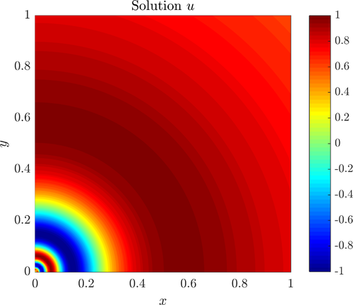
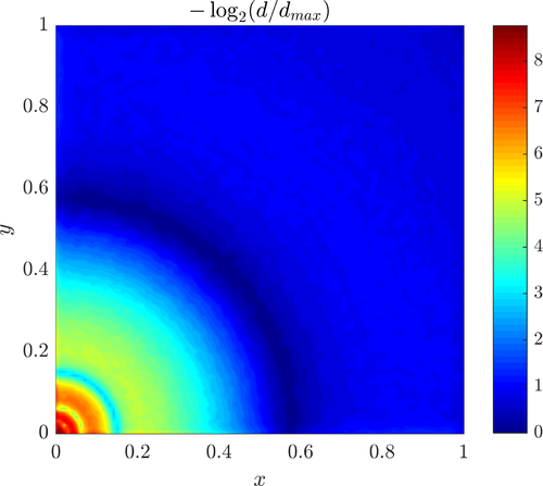
Solutions to many physical problems governed by partial differential equations (PDE) often significantly vary in magnitude throughout the problem domain. Although in some special cases the areas with high error are known in advance, in general the error distribution is unknown beforehand. Adaptive techniques for solving PDEs are a standard way of dealing with this problem, where problematic regions are iteratively refined. A step further is automatic adaptivity, where problematic regions are chosen automatically using an error indicator and then refined, until certain error threshold is reached. Below, we show some examples of fully automatic adaptivity in Medusa.
Contents
Basic concept
The adaptive methodology in this paper behaves similarly to "remeshing" used commonly in FEM. Some initial (possibly variable) nodal spacing $h^0$ is chosen, as well as its lower and upper bounds $h_L$ and $h_U$, respectively. 3 Domain $\Omega$ is filled with nodes, conforming to $h^0$ and the solution $u^0$ is obtained. An error indicator is employed to determine which nodes should be (de)refined and the nodal density $h^0$ is altered appropriately. This adaptive cycle below is repeated until the convergence criterion is met. The procedure on $j$-th iteration is written in more detail below:
- Fill $\Omega$ with nodes conforming to $h^j$.
- Solve the problem to obtain $u^j$.
- Compute the error indicator values $\varepsilon_i^j$ for each node $p_i$.
- If the mean of $\varepsilon_i^j$ is below some tolerance $\varepsilon$ return $u^j$ as the solution and stop.
- Adapt $h^j$ to obtain $h^{j+1}$.
More details can be found in our paper: https://arxiv.org/abs/1811.10368
Node density adaptation
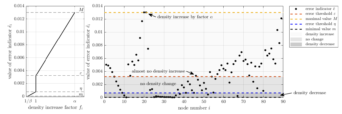
The existing nodal spacing function $h^j$ is evaluated at nodes $p_i$ to obtain values $h_{i,j} = h^j(p_i)$ . These values $h_{i,j}$ are modified by a density factor $f_i$ as $$ h_{i,j+1} = \min(\max(h_{i,j} / f_i, h_L(p_i)), h_U(p_i)), $$ where density factor $f_i$ is computed as $$ f_i = \begin{cases} 1 + \frac{\eta - \varepsilon_i}{\eta - m} (\frac{1}{\beta} - 1), & \varepsilon_i \leq \eta, \quad \text{i.e. decrease the density} \\ 1, & \eta < \varepsilon_i < \varepsilon, \quad \text{i.e. no change in density}\\ 1 + \frac{\varepsilon_i - \varepsilon}{M - \varepsilon} (\alpha - 1), & \varepsilon_i \geq \varepsilon, \quad \text{i.e. increase the density} \end{cases} $$ and $\alpha$ represents the refine aggressiveness, $\beta$ the derefine aggressiveness, $\varepsilon$ the refinement threshold, $\eta$ the derenfinement threshold, and $m = \min_i \varepsilon_i$ is the minimal and $M = \max_i \varepsilon_i$ is the maximal value of the error indicator. Note that setting $\alpha=1$ or $\beta=1$ disables refinement and derefinement, respectively.
This adaptation is illustrated in the figure below.
Error indicators
The work on error indicators is ongoing. For now, we use an ad hoc error indicator $$\varepsilon_i = \operatorname{std}_{j \in I_i}(u_j),$$ which represents the standard deviation of function values over all stencil nodes of a given node $p_i$.
Numerical exmaples
Below are several numerical examples where adaptivity has been tested or used to obtain solutions.
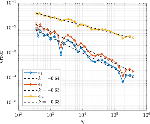
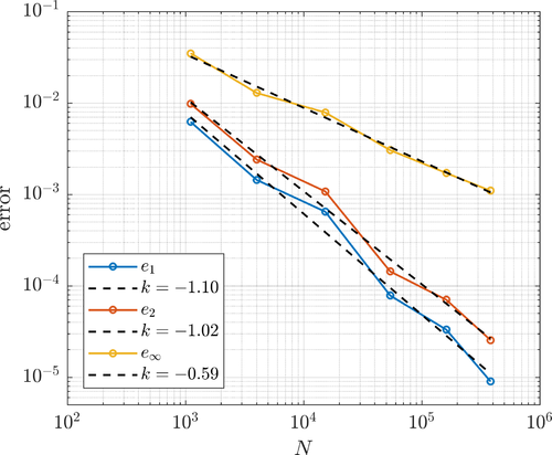
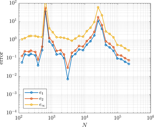
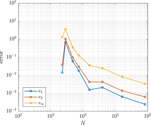
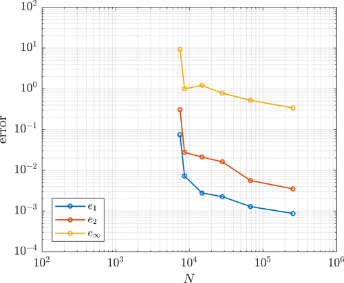
The errors $e_1$, $e_2$, $e_\infty$ and $e_E$ refer to relative discrete $L^1$, $L^2$, $L_\infty$ and energy norm errors, respectively. These are evaluated in the computation nodes or on a denser grid by reinterpolation.
L shaped domain
The L shaped domain problem is defined on $\Omega = [-1, 1]^2 \setminus [0, 1] \times [-1, 0]$. The Laplace problem $\nabla^2u = 0$ with the solution $u = r^{\frac{2}{3}} \sin(\frac{2}{3}\theta)$ given in polar coordinates.
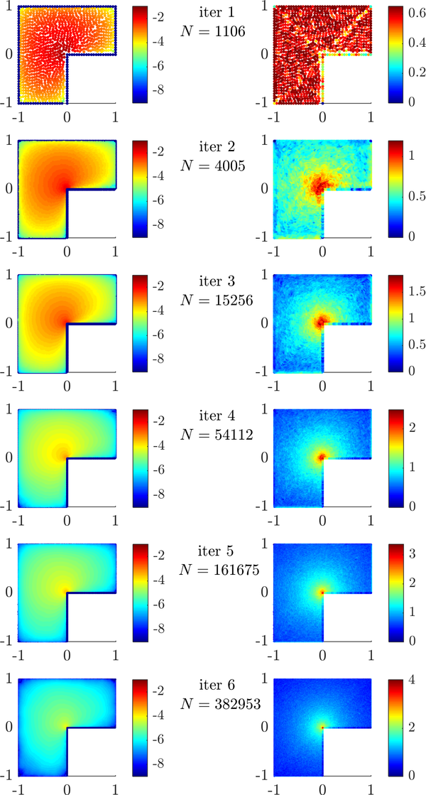
BF-FD method with Polyharmonic splines augmented with monomials up to and including 2nd order was used to approximate the differential operators. The stencils for each node were chosen by simply selecting the closest $n=15$ nodes. The resulting sparse system was solved using the Intel ® MKL Pardiso sparse solver. Both uniform and fully adaptive refinement was tested. The adaptive procedure was run with $\alpha=3$, $\varepsilon = 10^-2$, $\beta=1$ and $\eta=0$.
The errors under uniform (left) and adaptive (right) refinement are shown below.
The error (left) and the nodal density (right) during the adaptive iteration are shown below.
Disk under stress
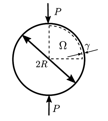
The next case is disk under pressure case from Linear elasticity solving the Caucy-Navier equation of Solid mechanics. The problem considers one quarter of the disk illustrated below by the domain $\Omega$. The spacing $\gamma$ represents the distance from the singularity.
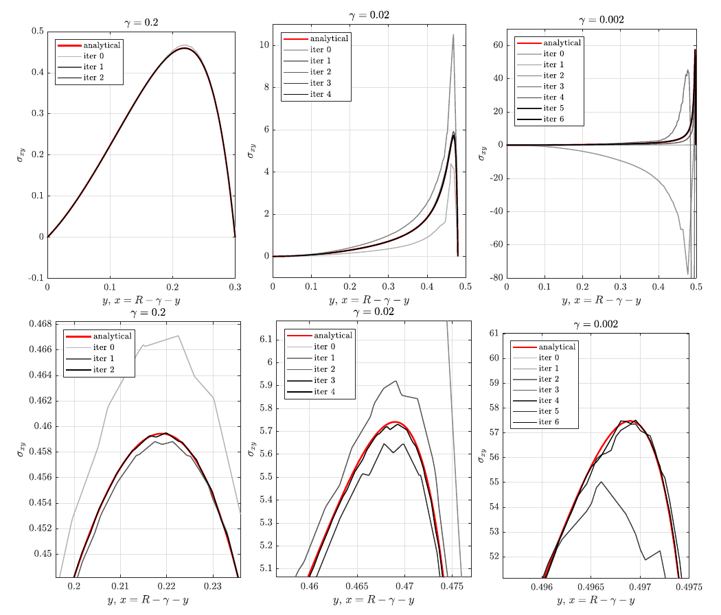
Computed $\sigma_{xy}$ stress profiles for three considered cases. The lower three images show close-ups of the computed peaks.
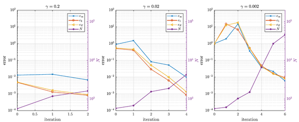
Error of the numerical solution of the compressed disk problem during adaptive iteration.
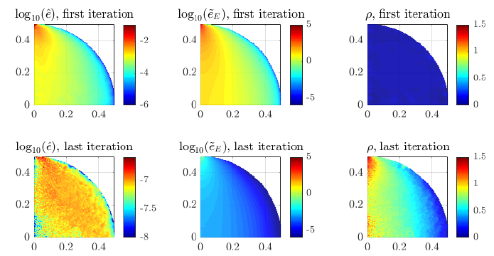
Error indicator value and node density in the last iteration.
Hertzian contact
Fretting fatigue contact
Bousinesq problem
Helmholz equation
Go back to Examples.
