Revision as of 20:58, 6 February 2017

Click here to return back to Solid Mechanics

Point contact on a 2D half-plane

A starting point to solve problems in contact mechanics is to understand the effect of a point-load applied to a homogeneous, linear elastic, isotropic half-plane. This problem may be defined either as plane stress or plain strain (for solution with FreeFem++ we have chosen the latter). The traction boundary conditions for this problem are: \begin{equation}\label{eq:bc} \sigma_{xy}(x,0) = 0, \quad \sigma_{yy}(x,y) = -P\delta(x,y) \end{equation} where $\delta(x,y)$ is the Dirac delta function. Together these boundary conditions state that there is a singular normal force $P$ applied at $(x,y) = (0,0)$ and there are no shear stresses on the surface of the elastic half-plane.

The analytical relations for the stresses can be found from the Flamant solution (stress distributions in a linear elastic wedge loaded by point forces a the tip. When the "wedge" is flat we get a half-plane. The derivation uses polar coordinates.) and are given as: \begin{equation} \sigma_{xx} = -\frac{2P}{\pi} \frac{x^2y}{\left(x^2+y^2\right)^2}, \end{equation} \begin{equation} \sigma_{yy} = -\frac{2P}{\pi} \frac{y^3}{\left(x^2+y^2\right)^2}, \end{equation} \begin{equation} \sigma_{xy} = -\frac{2P}{\pi} \frac{xy^2}{\left(x^2+y^2\right)^2}, \end{equation} for some point $(x,y)$ in the half-plane. From this stress field the strain components and thus the displacements $(u_x,u_y)$ can be determined. The displacements are given by \begin{align} u_x &= -\frac{P}{4\pi\mu}\left((\kappa-1)\theta - \frac{2xy}{r^2}\right), \label{eq:dispx}\\ u_y &= -\frac{P}{4\pi\mu}\left((\kappa+1)\log r + \frac{2x^2}{r^2}\right), \label{eq:dispy} \end{align} where $$r = \sqrt{x^2+y^2}$$ and $$\tan \theta = \frac{x}{y}.$$ The symbol $\kappa$ is known as Dundars constant and is defined as \[ \kappa = \begin{cases} 3 - 4\nu & \quad \text{(Plane strain)}, \\ \cfrac{3 - \nu}{1+\nu} & \quad \text{(Plane stress)}. \end{cases} \] The last remaining symbol is $\mu$ which represents the shear modulus (sometimes also denoted with $G$).

Numerical solution with FreeFem++

Due to the known analytical solution the point-contact problem can be used for benchmarking numerical PDE solvers in terms of accuracy (as well as computational efficiency). The purpose of this section is to compare the numerical solution obtained by FreeFem++ with the analytical solution, as well as provide a reference numerical solution for the C++ library developed in our laboratory.

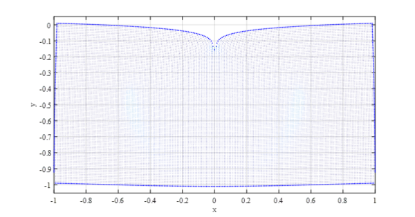
For purposes of simplicity we limit ourselves to the domain $(x,y) \in \Omega = [-1,1] \times[-1,-0.1]$ and prescribe Dirichlet displacement on the boundaries $\Gamma_D$ from the known analytical solution (\ref{eq:dispx}, \ref{eq:dispy}). This way we avoid having to deal with the Dirac delta traction boundary condition (\ref{eq:bc}). The problem can be described as find $\boldsymbol{u(\boldsymbol{x})}$ that satisfies \begin{equation} \boldsymbol{\nabla}\cdot\boldsymbol{\sigma}= 0 \qquad \text{on }\Omega \end{equation} and \begin{equation} \boldsymbol{u} = \boldsymbol{u}_{\text{analytical}} \qquad \text{on }\Gamma_D \end{equation} where $\boldsymbol{u}_\text{analytical}$ is given in equations (\ref{eq:dispx}) and (\ref{eq:dispy}).

To solve the point-contact problem in FreeFem++ we must first provide the weak form of the balance equation: \begin{equation*} \boldsymbol{\nabla}\cdot\boldsymbol{\sigma} + \boldsymbol{b} = 0. \end{equation*} The corresponding weak formulation is \begin{equation}\label{eq:weak} \int_\Omega \boldsymbol{\sigma} : \boldsymbol{\varepsilon}(\boldsymbol{v}) \, d\Omega - \int_\Omega \boldsymbol{b}\cdot\boldsymbol{v}\,d\Omega = 0 \end{equation} where $:$ denotes the tensor scalar product (tensor contraction), i.e. $\boldsymbol{A}:\boldsymbol{B} =\sum_{i,j} A_{ij}B_{ij}$. The vector $\boldsymbol{v}$ is the test function or so-called "virtual displacement".

Equation (\ref{eq:weak}) can be handed to FreeFem++ with the help of Voigt or Mandel notation, that reduces the symmetric tensors $\boldsymbol{\sigma}$ and $\boldsymbol{\varepsilon}$ to vectors. The benefit of Mandel notation is that it allows the tensor scalar product to be performed as a scalar product of two vectors. For this reason we create the following macros:

 macro u [ux,uy] // displacements
 macro v [vx,vy] // test function
 macro b [bx,by] // body forces
 macro e(u) [dx(u[0]),dy(u[1]),(dx(u[1])+dy(u[0]))/2] // strain (for post-processing)
 macro em(u) [dx(u[0]),dy(u[1]),sqrt(2)*(dx(u[1])+dy(u[0]))/2] // strain in Mandel notation
 macro A [[2*mu+lambda,mu,0],[mu,2*mu+lambda,0],[0,0,2*mu]] // stress-strain matrix

The weak form (\ref{eq:weak}) can then be expressed naturally in FreeFem++ syntax as int2d(Th)((A*em(u))'*em(v)) - int2d(Th)(b'*v)

Explicit solution with Meshless Local Strong Form Method (MLSM)

 1     RectangleDomain<vec_t> domain(O.domain_lo, O.domain_hi);
 2     domain.fillUniformInteriorWithStep(O.d_space);
 3     domain.fillUniformBoundaryWithStep(O.d_space);
 4     domain.findSupport(O.n, internal);
 5     domain.findSupport(O.n, boundary, internal, true);
 6 
 7     EngineMLS<vec_t, Gaussians, Gaussians> mls(
 8         {pow(domain.characteristicDistance()*O.sigmaB,2), O.m},  
 9         domain.positions[domain.support[0]],
10         pow(domain.characteristicDistance()*O.sigmaW,2));       
11     auto mlsm = make_mlsm(domain, mls, internal);
12     for (auto& i : boundary)    u_3[i]  = u_anal(i);
13     /// [MAIN TEMPORAL LOOP]
14     for (size_t step = 0; step * O.dt < O.time; step++) {
15         int i;  
16         ///[NAVIER-CAUCHY EQUATION :: explicit Plane Stress]
17         #pragma omp parallel for private(i) schedule(static)
18         for (i=0;i<internal.size();++i){
19             u_3[i] = O.dt * O.dt / O.rho * (
20                     O.mu * mlsm.lap(u_2,i) + O.E/(2-2*O.v ) 
21                     * mlsm.graddiv(u_2,i) +
22                     force[i] - O.dampCoef * (u_2[i] - u_1[i])/O.dt
23                 ) /// navier part
24                 + 2 * u_2[i] - u_1[i];   
25         }
26         ///[STEP FORWARD]
27         u_1 = u_2;
28         u_2 = u_3;
29 }

Note that an operator grad(div(u)) that requires also mixed derivatives is used. To obtain stable solution a minimal second order monomial basis is required.

Implicit solution with Meshless Local Strong Form Method (MLSM)

 1     /// [Field declarations]
 2     Eigen::SparseMatrix<double, Eigen::RowMajor> M(2 * N, 2 * N);
 3 
 4     Range<int> tmp(2 * N, O.n);
 5     M.reserve(Range<int>(2 * N, O.n));
 6     Eigen::VectorXd rhs(2 * N);
 7 
 8     // Set equation on interior
 9     for (int i : internal) {
10         op.lapvec(M, i,  O.E / (2 + 2 * O.v));
11         op.graddiv(M, i, O.E / (2 - 2 * O.v));  // graddiv + laplace in interior
12         rhs(i) = 0;
13         rhs(i+N) = 0;
14     }
15     // Set boundary conditions
16     for (int i : boundary) {
17         M.coeffRef(i, i) = 1;  // boundary conditions on the boundary
18         M.coeffRef(i+N, i+N) = 1;  // boundary conditions on the boundary
19         Vec2d bc = analytical(i);
20         rhs(i) = bc[0];
21         rhs(i+N) = bc[1];
22     }
23 
24     // Sparse solve
25     Eigen::BiCGSTAB<Eigen::SparseMatrix<double, Eigen::RowMajor>> solver;
26     solver.setTolerance(1e-15);
27     solver.compute(M);
28     Eigen::VectorXd sol = solver.solve(rhs);

Results

Purely Dirichlet case

For starters we check the solution of the problem with Dirichlet BC. The conditions are obtained from closed form solution #Point contact on a 2D half-plane.

The $L^2$ error norm is used to quantify the error. Since the displacements are the variable that obtain from FreeFem++, we use the displacement magnitude $\|\boldsymbol{u}\| = \sqrt{u_x^2+u_y^2}$ to define our $L^2$-error norm. We first define the relative error field:

\begin{equation} L^2(\b{x}_i) = \frac{\|\b{u}(\b{x}_i)-\b{u}_\text{analytical}(\b{x}_i)\|}{\mathrm{max}\left(\| \b{u}_\text{analytical}(\b{x}_i)\| ,10^{-10}\right)}, \end{equation}

and then take the maximum $L^2$ error as our indicator:

\begin{equation} L^2 = \mathrm{max}_i\left(L^2(\b{x}_i)\right) \end{equation}

For the FreeFem++ convergence test we vary the number of nodes by increasing the square grid size in both $x$- and $y$- directions simultaneously by powers of two from $2^2$ (16 nodes all together) to $2^7$ (16384 nodes all together).

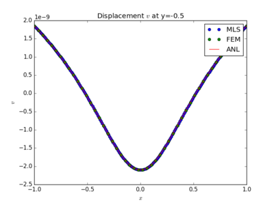
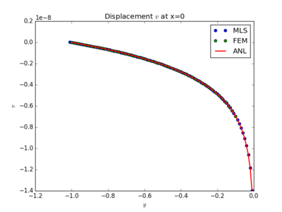
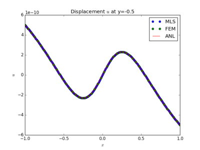
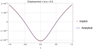
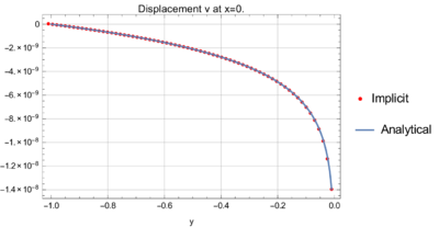
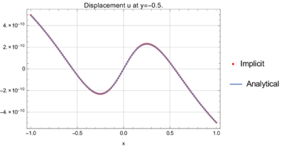
Comparison of MLS based explicit and implicit MLSM, FEM and analytical solution of displacements at different cross-sections.

Convergence

FEM (1) MLSM explicit (2) and implicit (3) convergence

FEM Convergence results for the point contact problem. The colours blue, red and green represent linear, quadratic and cubic finite elements, respectively. 400px 500px

Note, that this are preliminary results and there might be some minor mistakes. Updates coming soon :)