Difference between revisions of "Refinement of the nodal distribution"

Revision as of 10:17, 15 September 2020

Here we consider possible meshless refinement algorithms (sometimes also called adaptive cloud refinement). The refinement mechanisms we have so far studied include:

• refinement based on closest node distance
• refinement based on averaged (inter-)node distance
• refinement based on half-links

Here we only want to compare the quality of the refined grids and have not tied the refinement algorithm with a error indicator, thus we only study the node insertion process by refining the whole grid.

The refinement routine takes a range of nodes (e.g. a subregion of the domain) together with the refinement parameters and generates new nodes around the old ones. Special care must be taken with refinement of the boundary nodes. Points have to be selected on the actual boundary either analytically considering the geometry or with a numerical root finder such as bisection.

Problem description

To compare the node refinement mechanisms we study the process of reaction-diffusion in an infinite cylindrical catalyst pellet (infinite in the $z$-dimension). Since the pellet is infinite in one dimension this problem simplifies to a 2D problem (in the $xy$-plane). For a catalyst pellet of radius $R$ centered at $(x,y) = (0,0)$ and the reactant undergoing a first order reaction we must solve the equation \begin{equation} \b{\nabla}^2 C - {M_T}^2 C = 0, \end{equation} where $C$ is the concentration of the reactant, $M_T = R\sqrt{k/D}$ is known as Thiele's modulus and $k$ and $D$ represent the reaction rate constant and diffusivity of the reacting species. The boundary conditions for this problem is \[C(R) = C_s.\] The analytical solution can be found easily using cylindrical coordinates and is given by \begin{equation} \frac{C(r)}{C_S} = \frac{I_0(r M_T)}{I_0(R M_T)}, \end{equation} where $I_0(r)$ is the modified Bessel function of first kind (this function is available in the library Boost as well as scripting languages such as Python or MATLAB). The conversion from cartesian to cylindrical coordinates is given by \[r = \sqrt{x^2+y^2}.\]

Error indicators

To compare the quality of the refined meshes for the described problem case we look at different error criteria including the max norm $L_\infty$ defined as \begin{equation} L_\infty = \mathrm{max}_i \left|C_i^\mathrm{numerical} - C_i^\mathrm{analytical}\right|, \end{equation} the $L_2$ norm per node defined as \begin{equation} \bar{L_2} = \frac{\sqrt{\sum^N_{i = 1}\left(C_i^\mathrm{numerical} - C_i^\mathrm{analytical}\right)^2}}{N}, \end{equation} where $N$ is the number of nodes (and pertinent equations) in the domain.

We also measure the number of iterations required by the sparse BiCGSTAB solver to reach convergence and the estimated error of solving the system of equations.

Closest node

For a given node $\b{x}_0 = (x_0,y_0)$:

1. find the closest node $\b{x}_1 = (x_1,y_1)$
2. calculate the half distance between the two nodes \[d = |\b{x}_1 - \b{x}_0|/2\]
3. randomly select up to 6 (The case of 6 nodes is the limit since it produces a regular hexagon. In practice this never occurs due to the "monte carlo" node selection procedure.) new nodes on the circle with center $\b{x}_0$ and radius $d$ and simultaneously make sure their is a minimal inter-nodal distance $d$ between the new nodes.

For boundary points we first select 2 points that intersect with the boundary of the domain and only then points lying inside the domain. Due to geometrical constraints boundary points will usually end up with 3 new nodes (in case of straight boundaries we could end up with 4, which would be the previously discussed hexagon limit).

Figure 1: Refinement based on closest node approach (initial unrefined grid is on the left). In the second refinement step an erroneous point has appeared from an internal point that was too close to the boundary. Also noticable is clustering of points on the boundary.

Average radius

Input parameters: $f$ and $l_s$

For a given node $\b{x}_0$:

1. find the $l_s$ (an integer from 1 to 7) closest nodes
2. calculate the average distance $\bar{d}$ to the $l_s$ closest nodes
3. randomly select up to 6 new nodes on the circle with center $\b{x}_0$ and radius $f\cdot\bar{d}$ where $f$ is the radius fraction that lies between 0.2 (leads to clustering) and 0.8. Only allow nodes that are separated by the distance $f \cdot \bar{d}$.

(note that in case $l_s = 1$ and $f = 0.5$ the average radius mechanism becomes equal to the closest node refinement approach described above)

Figure 2: Refinement based on average radius approach (initial unrefined grid is on the left). The parameters are $l_s = 5$ closest nodes in average radius calculation and points placed at radius fraction $f = 0.5$.

Half-links

Warning: this is still a prototype

Input parameters: $l_s$, $d_m$

For a given node $\b{x}_0$:

1. find the $l_s$ (an integer from 1 to 7) closest nodes $\b{x}_i$
2. select new nodes in the middle of the segments $\b{x}_i - \b{x}_0$ only allowing points that are separated by the minimal distance $d_m$

(note also that in the 1D case the half-link and closest radius approach become the same)

The minimal distance $d_m$ is chosen as a fraction of the distance to the closest link, e.g. $d_m = f d$, where $f$ is the provided fraction and $d$ is the distance to the closest link.

Figure 3: Refinement based on half links (initial unrefined grid is on the left). The parameters are $l_s = 6$ and $d_m = 0.4 d$, where $d$ is the distance to the closest link.

Figure 4: Refinement based on half links with additional 10 step relax after refinement

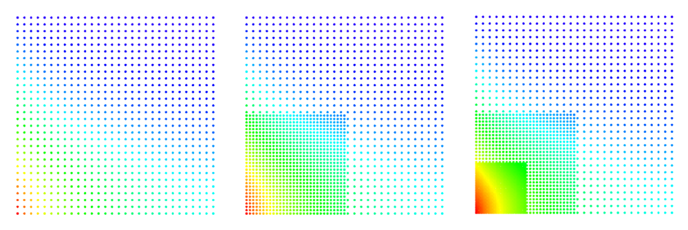
After experimentation we noticed there are some inconsistencies when trying to refine structured point sets with this approach. The reason for these inconsistencies is that the boundary and internal points have a different number of "natural neighbours". For example in 2D on a square grid, the internal points have 8 neighbours, while boundary points have 5 neighbours. If we choose higher numbers e.g 9 links for an internal node, the 9th node might be any of the 4 nodes one shell further out that only differ at machine precision.

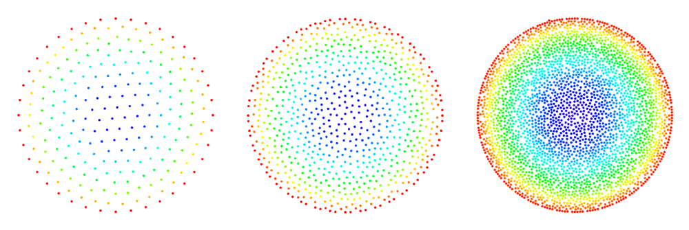
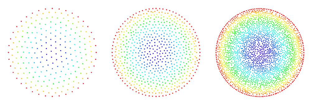
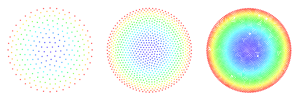
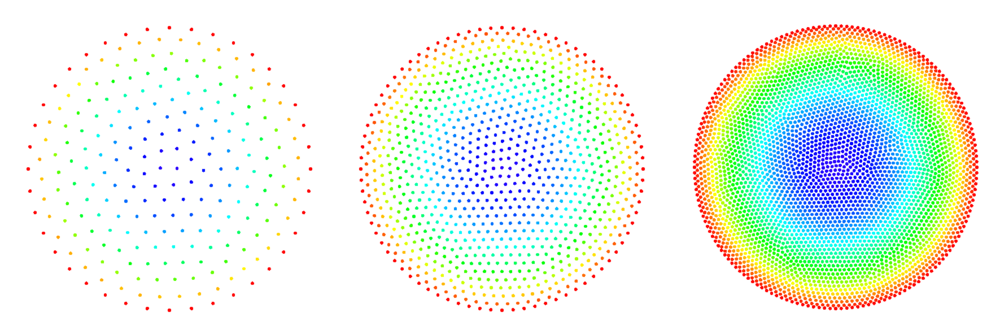
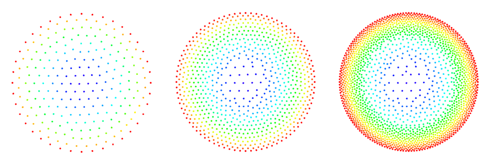
The figures below show some preliminary results of refinement based on half-links. For the circle domain relaxation was applied after the refinement.

Figure 5: Thermal diffusion in (convective) flow at a stagnation point (bottom left corner).

After the second refinement of the corner, the solver had difficulty converging to the solution. This was the result of a fixed size shape parameter in the shape functions of the node points. The shape functions have to be tailored to the local characteristic distance in the point set.

Figure 6: Reaction-diffusion in a cylinder catalyst. Two successive refinements have been applied for $r > 0.5$ and $r > 0.8$, where $r$ is the radial coordinate. The cylinder radius $R = 1$.$

Hybrid approach

A hybrid might give better distributions of the refined points. The half-link approach performs well at the boundaries while the distance approach gives less regular internal distributions. In any case it is suggested to perform a few more relaxation steps to equilibrate the mesh.

Figure 7: Refinement based on half links at the boundaries and closest distances for the internal nodes (initial unrefined grid is on the left). for the boundary nodes the parameters are $l_s = 7$ and $d_m = 0.5 d$, where $d$ is the distance to the closest link.