Difference between revisions of "Heat equation"
| Line 84: | Line 84: | ||
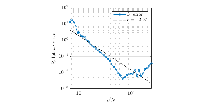
We ran simulation a couple of times using different dx values. Changing dx value changed number of total nodes as well. We made logarithmic graph of relative error per number of nodes. | We ran simulation a couple of times using different dx values. Changing dx value changed number of total nodes as well. We made logarithmic graph of relative error per number of nodes. | ||
| + | |||
| + | [[File:error_total_nodes.png|800px]] | ||
Go back to [[Medusa#Examples|Examples]]. | Go back to [[Medusa#Examples|Examples]]. | ||
Revision as of 15:16, 19 August 2019
Go back to Examples.
Purpose of Heat equation example
This example shows how explicit method of solving partial differential equations is used within the medusa library. Firstly, this example compares explicit solutions to analytical, then it shows how it can be used to solve heat transfer equation.
Domain
In this example, a square domain with a cut-out hole in the middle is used. The hole has radius equal to 1/3 of length of a square. Domain nodes are placed randomly with about dx length distance between them.
1 BoxShape<Vec2d> box(-3.0, 3.0);
2 DomainDiscretization<Vec2d> domain=box.discretizeBoundaryWithStep(dx);
3 BallShape<Vec2d> ball(0,1.0);
4 DomainDiscretization<Vec2d> domain_empty=ball.discretizeBoundaryWithStep(dx,-5);
5 domain -=domain_empty;
6 GeneralFill<Vec2d> fill_engine;
7 fill_engine(domain, dx);
Domain boundary is separated in to 5 areas: up, down, left, right and center.
1 auto internal = domain.interior();
2 auto up = domain.types().filter([](int i) { return i == -4 ; });
3 auto down = domain.types().filter([](int i) { return i == -3 ; });
4 auto right = domain.types().filter([](int i) { return  i == -2; });
5 auto left = domain.types().filter([](int i) { return  i == -1; });
6 auto center=domain.types().filter([](int i){ return i == -5;});
The idea of this domain is to have Dirichlet boundary condition on the square. Furthermore, they are constant over the course of simulation. In the center, the boundary conditions are Neumann.
Fuction, solution and comparison
The function used for this example is $u(x,y) = \sin(\pi x)\sin(\pi y)$. Laplace operator of this function is $\Delta u(x,y)=-2\pi^2\sin(\pi x)\sin(\pi y)$. For comparing explicit solution to analytical, we solve function for each node and save solution to u1_analytic. With this we also calculate Dirichlet boundary conditions. Then we set interior and center of domain to arbitrary value, in this case 0. Then we proceed to explicitly solve the domain interior and center. In the domain interior we are solving the following equation\[ \begin{align*} u (x,y,t+1) = dt*\bigg(\Delta u(x,y,t) + 2\pi^2\sin(\pi x)\sin(\pi y)\bigg)+u(x,y,t) \end{align*} \]
For domain center we set value of $u(x,y,t+1)$ in a way that it satisfies the following equation\[ \frac{\partial u(x,y,t+1)}{\partial n}=n_x \pi \cos(\pi x) \sin(\pi y)+n_y \pi \sin(\pi x) \cos(\pi y) \]
While doing this, we also compare previous values u1 to new ones u2. If there are differences bigger than dt*1E-5, we continue the simulation. Otherwise, we stop it and compare values in nodes to analytical ones.
 1 while (ending){
 2         if (iteracije%izpis==0) {
 3             std::cout << iteracije << std::endl;
 4         }
 5         iteracije++;
 6 #pragma omp parallel for
 7         for (int j = 0; j < internal.size(); ++j) {
 8             int i = internal[j];
 9             u2[i] = dt *( op.lap(u1, i) +2*PI*PI*function(domain.pos(i,0),domain.pos(i, 1)))+ u1[i];
10         }
11 #pragma omp parallel for
12         for (int j = 0; j < center.size(); ++j) {
13             int i = center[j];
14             auto vec=domain.normal(i);
15             double x=domain.pos(i,0);
16             double y=domain.pos(i, 1);
17             u2[i]=op.neumann(u1,i,vec,vec[0]*PI*cos(PI*x)*sin(PI*y)+vec[1]*PI*cos(PI*y)*sin(PI*x));
18         }
19         for (int i:internal+center){
20             double razlika=abs(u1[i]-u2[i]);
21             if (razlika>konec){
22                 break;
23             }
24             ending = false;
25         }
26         u1.swap(u2);
27     }
We ran simulation a couple of times using different dx values. Changing dx value changed number of total nodes as well. We made logarithmic graph of relative error per number of nodes.
Go back to Examples.
