Latest revision as of 07:46, 15 December 2017

Click here to return back to Fluid Mechanics

Introduction

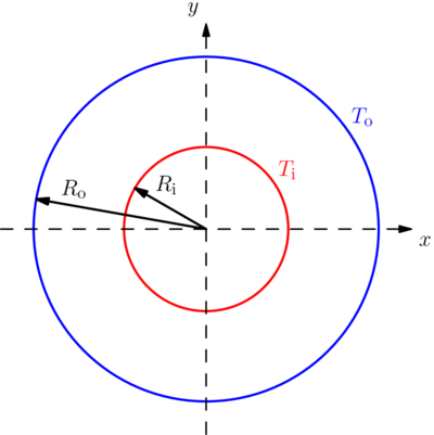
Another classical fluid flow benchmark is that of natural convection heat transfer in the annular space between concentric cylinders. This problem was first studied numerically by Kuehn and Goldstein (1975) using a stream function-vorticity formulation of the Navier-Stokes equations. Several assumptions are made in specifying the problem. First of all the flow is assumed to be invariant along the axis of the cylinders which leads to a two-dimensional flow configuration as schematically shown in the figure below. A constant property Boussinesq approximation is used. The buoyancy force may then be given as: \begin{equation} \b{g} = \left(\begin{matrix}g_x \\ g_y \end{matrix}\right) = \left(\begin{matrix}0 \\ g \beta \left(T - T_\mathrm{o}\right) \end{matrix}\right) \label{buoyancy} \end{equation} where $g$ is the gravitational acceleration, $T$ the temperature at a point within the fluid, $T_\mathrm{o}$ the temperature of the outer cylinder and $\beta$ the thermal volumetric expansion coefficient. The inner cylinder is held at a constant temperature $T_\mathrm{i}$.

Figure 1: Schematic diagram for the concentric cylinder geometry.

Governing equations

To solve this problem we will use the same formulation as Kuehn and Goldstein (1975) only that we will use MLSM to supply the discrete approximations to the PDE operators. Note that in the actual computations it is convenient to use the velocities $\b{v} = \left(u, v\right)^T$ rather than the derivatives of the stream function in the coefficients. The equations to be solved are: \begin{equation} \Delta \psi = \omega \end{equation} \begin{equation} \frac{\partial \omega}{\partial t} + u\frac{\partial \omega}{\partial x} + v\frac{\partial \omega}{\partial y} = \nu \Delta \omega + \left(\frac{\partial g_x}{\partial y} - \frac{\partial g_y}{\partial x}\right) \end{equation} \begin{equation} \rho c\frac{\partial T}{\partial t} + \b{v}\cdot\nabla T = k \Delta T \end{equation}

with knowing that \begin{equation} \b{v}=\nabla \times \psi \end{equation} and having in mind that we are dealing with 2D problem.

The fluid properties that appear in this problem are the fluid density $\rho$, specific heat $c$, kinematic viscosity $\nu$ and thermal conductivity $k$. The equations can be put into dimensionless form by introducing the following new variables:

\[t' = \frac{\alpha t}{L^2}, \quad x' = \frac{x}{L}, \quad y' = \frac{y}{L}, \quad \phi = \frac{T- T_\mathrm{o}}{T_\mathrm{i}-T_\mathrm{o}}, \quad u' = \frac{uL}{\alpha}, \quad v' = \frac{vL}{\alpha}, \quad \omega' = \frac{L^2}{\alpha}\omega, \quad \psi' = \frac{\psi}{\alpha}\] where $L = R_\mathrm{o} - R_\mathrm{i}$ is the gap between cylinders and $\alpha = k/(\rho c)$ is the thermal diffusivity. Upon inserting the buoyancy term \eqref{buoyancy}, substituting with the dimensionless variables and dropping the prime $'$ for simplicity, the dimensionless equations are: \begin{equation} \Delta \psi = \omega \end{equation} \begin{equation} \frac{\partial \omega}{\partial t} + \b{v}\cdot\nabla\omega = \mathit{Pr} \Delta \omega + \mathit{Ra}_L \mathit{Pr} \frac{\partial \phi}{\partial x} \end{equation} \begin{equation} \frac{\partial \phi}{\partial t} + \b{v}\cdot\nabla\phi = \Delta \phi \end{equation}

The dimensionless variables that appear in these equations are the Prandtl number \[ \mathit{Pr} = \frac{\mu c}{k} = \frac{\nu}{\alpha} \] and the Rayleigh number \[ \mathit{Ra}_L = \frac{g \beta \left(T_\mathrm{i} - T_\mathrm{o}\right)L^3}{\nu \alpha} \]

Boundary conditions

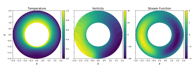
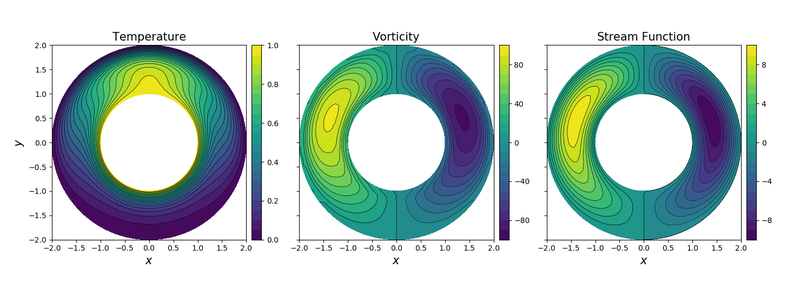
The boundary conditions that appear in this problem are two impermeable isothermal walls at constant radii. The stream function $\psi$ is constant along each wall. Since no flow enter or escapes form the enclosure, the stream function is set equal to zero on all boundaries. The dimensionless temperature equals unity on the inner cylinder and zero on the outer cylinder. The value of the vorticity at the boundaries may be found by directly applying \[ \omega = \Delta \psi \] along the walls.

The boundary condition are therefore \begin{equation} \psi = u = v = 0, \quad \omega = \Delta \psi, \quad \phi = 1 \end{equation} on the inner cylinder and \begin{equation} \psi = u = v = 0, \quad \omega = \Delta \psi, \quad \phi = 0 \end{equation} on the outer cylinder.

Code

A snippet of MLSM code for the stream function - vorticity approach looks like: (full examples will be available soon under the examples folder in the code repository Main Page).

 1     // Boundary Conditions
 2     T2[inner] = 1.0;
 3     T1 = T2;
 4 
 5     // Poisson equation matrix
 6     SparseMatrix<double, RowMajor> M_scal(size,size);
 7     M_scal.reserve(Range<int>(size,n));
 8     BiCGSTAB<SparseMatrix<double, RowMajor>> solver;
 9     VecXd rhs(size,0);
10     for (int c : boundary) op.value(M_scal, c, 1.0);
11     for (int c : interior) op.lap(M_scal, c, 1.0);
12     M_scal.makeCompressed();
13     solver.compute(M_scal);
14 
15     // Vorticity transport equation
16     auto derivative_W = [&](double, const Eigen::VectorXd& w) {
17         Range<double> rw = reshape(w);
18         Range<double> der(rw.size(), 0);
19         int i;
20         #pragma omp parallel for private(i) schedule(static)
21         for (i = 0; i < interior.size(); ++i) {
22             int c = interior[i];
23             der[c] = Pr*op.lap(rw, c) + Ra*Pr*op.grad(T2,c)[0] - U[c].dot(op.grad(rw,c));
24         }
25         return reshape(der);
26     };
27 
28     // Temperature equation
29     auto derivative_T = [&](double, const VecXd& T) {
30         VecXd der = Eigen::VectorXd::Zero(T.size());
31         int i;
32         #pragma omp parallel for private(i) schedule(static)
33         for (i = 0; i < interior.size(); ++i) {
34             int c = interior[i];
35             der[c] = op.lap(T, c) - U[c].dot(op.grad(T, c));
36         }
37         return der;
38     };
39 
40     auto integrator_W = integrators::Explicit::RK4().solve(derivative_W, 0.0, time, dt, reshape(W1));
41     auto integrator_T = integrators::Explicit::RK4().solve(derivative_T, 0.0, time, dt, reshape(T1));
42 
43     auto W_stepper = integrator_W.begin();
44     auto T_stepper = integrator_T.begin();
45 
46     for (int step = 0; step <= t_steps; ++step) {
47 
48         // Poisson equation for stream function
49         for (auto c : interior) {
50             rhs[c] = W1[c];
51         }
52         PSI = reshape(solver.solveWithGuess(rhs, reshape(PSI)));
53 
54         // Calculate velocity
55         for (auto c : interior) {
56             vec_t grad_psi = op.grad(PSI,c);
57             U[c] = vec_t{grad_psi[1],-grad_psi[0]};
58         }
59 
60         ++T_stepper;
61         T2 = reshape(T_stepper.value());
62 
63         // Apply vorticity BC
64         for (auto c : boundary) {
65             W1[c] = op.lap(PSI,c);
66         }        
67         ++W_stepper;
68         W2 = reshape(W_stepper.value());
69 
70 
71         W1.swap(W2);
72         T1.swap(T2);
73     }

Results

Sources

Kuehn, T. H., & Goldstein, R. J. (1976). An experimental and theoretical study of natural convection in the annulus between horizontal concentric cylinders. Journal of Fluid mechanics, 74(4), 695-719.