Difference between revisions of "Lid driven cavity"
(→Results) |
(→Results) |
||
| Line 34: | Line 34: | ||
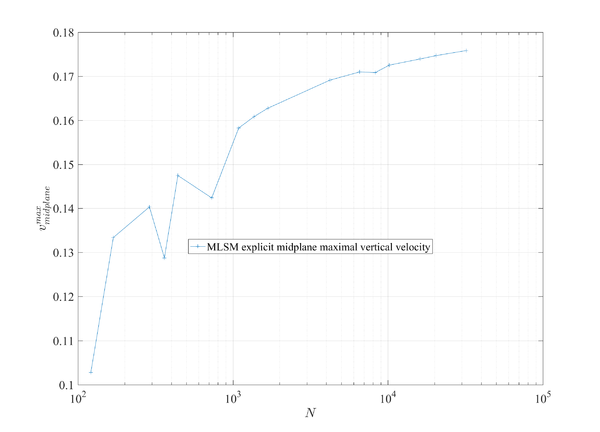
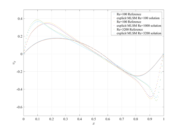
| − | + | [[File:lid_driven_explicit_exec_time.png|600px]][[File:lid_driven_explicit_convergence.png|600px]] | |
| − | |||
| − | |||
| − | |||
| − | |||
| − | |||
| − | |||
| − | |||
| − | |||
| − | |||
| − | |||
| − | |||
| − | [[File:lid_driven_explicit_exec_time.png|600px]] | ||
| − | |||
| − | |||
| − | |||
| − | |||
| − | [[File:lid_driven_explicit_convergence.png|600px]] | ||
| − | |||
| − | |||
Revision as of 19:55, 22 October 2017
Intro
back to Fluid Mechanics
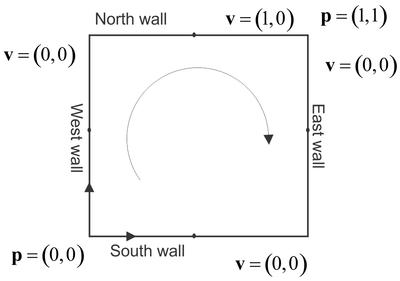
Let's try MLSM and described solution procedures first on a lid driven cavity problem that stands for a standard benchmark test for validation of the fluid flow solvers. It has been proposed in 1982 and since then solved by many researchers with wide spectra of different numerical methods. The test is still widely studied and used for validation of novel methods and numerical principles. Case is schematically presented in Figure 1 followed by few basic analyses, just to show that things work as they should. Details about comparison can be found in paper
Code
The snippet of the MLSM code for an explicit ACM method with CBS looks like: (full examples, including implicit versions, can be found under the examples in the code repository Main Page).
 1     for (int step = 0; step <=O.t_steps; ++step) {
 2         // Navier-Stokes
 3         for (auto i:interior)
 4             // Navier-Stokes
 5             v2[c] = v1[c] + O.dt * ( - 1/O.rho    * op.grad(P1,c)
 6                                      + O.mu/O.rho * op.lap(v1, c)
 7                                      -              op.grad(v1,c)*v1[c]);
 8         }
 9         // Mass continuity
10         for (auto i:interior) {
11             P2[i] = P1[i] - O.dl * O.dt * O.rho * op.div(v2,i) + O.dl2 * O.dl * O.dt * O.dt * op.lap(P1,i);
12         }
13         v1.swap(v2);
14         P1.swap(P2);
15     }
Results
