Difference between revisions of "Solving sparse systems"
Mitjajancic (talk | contribs) |
Mitjajancic (talk | contribs) (Added some observations.) |
||
| Line 133: | Line 133: | ||
The condition number iz arther large and grows superlinearly with size in the example below. | The condition number iz arther large and grows superlinearly with size in the example below. | ||
[[File:cond.png|600px]] | [[File:cond.png|600px]] | ||
| − | |||
| − | |||
| − | |||
| − | |||
| − | |||
| − | |||
| − | |||
| − | |||
| − | |||
| − | |||
| − | |||
| − | |||
| − | |||
| − | |||
| Line 170: | Line 156: | ||
* [https://eigen.tuxfamily.org/dox/classEigen_1_1PardisoLU.html PardisoLU]. | * [https://eigen.tuxfamily.org/dox/classEigen_1_1PardisoLU.html PardisoLU]. | ||
| − | The performance tests are focused on the accuracy of the numerical solution, number of iterations and time required to solve the final sparse system. We also comment on the amount of RAM required by a specific solver. | + | The performance tests are focused on the accuracy of the numerical solution, number of iterations and time required to solve the final sparse system. We also comment on the amount of RAM required by a specific solver. If required, the [https://gitlab.com/e62Lab/eigen_solvers_analysis gitlab repository] with the implementation is also provided. |
| Line 200: | Line 186: | ||
Example solutions to both scenarios are shown in figure below. | Example solutions to both scenarios are shown in figure below. | ||
| − | [[File:solution_poisson. | + | [[File:solution_poisson.png|800px]] |
| + | |||
| + | === Solver performance === | ||
| − | + | Below, we show the performance of the selected solvers in case of a two-dimensional Poisson problem. The first column shows the accuracy of the numerical solution in terms of the infinity norm, the second column shows the number of iterations a given solver required (direct solvers were assigned a value 1) and the third column shows the total time required to solve the system and obtain the numerical solution $\widehat u$. | |
| − | + | <syntaxhighlight lang="text"> | |
| − | + | Computational times: To obtain the computational times the code was run on a single CPU with assured CPU affinity using the ''taskset'' command. | |
| − | + | </syntaxhighlight> | |
| − | |||
| − | + | [[File:convergence_poisson_sin.png|1200px]] | |
| − | |||
| − | |||
| − | |||
| + | [[File:convergence_poisson_exp.png|1200px]] | ||
| − | + | In terms of accuracy, all solvers under consideration perform equally good, with an exception of BiCGSTAB with ILUT preconditioner, who failed to obtain a solution of sufficient accuracy at the finest domain discretization with approximately $2\cdot 10^6$ nodes. The reason is most likely in the ILUT preconditioner, set to limit solver iterations to 200 with fill factor 40, drop tolerance $10^{-5}$ and global tolerance $10^{-15}$. A different ILUT setup would most probably yield a more desirable behaviour, but it nevertheless shows that when using a ILUT preconditioner one must be careful before making conclusions. It is also important to note that the SparseLU ran out of the available 11.5 Gb RAM and, therefore, failed to obtain a numerical solution. Other solvers had no issues with the available RAM space. | |
| − | |||
| − | + | It is perhaps more interesting to study the number of iterations required by the solvers. Obviously, direct solvers require a "single iteration". Iterative solvers, on the other hand, require multiple iterations. Generally speaking, we observe that the number of solver iterations increases with the number of discretization points. However, it is interesting to see that the pure BiCGSTAB shows the most stable and predictable behaviour. Despite the fact that the guess provided to the BiCGSTAB is in fact the analytical solution to the problem, we do not observe significantly lower number of solver iterations. | |
| − | |||
| − | |||
| − | |||
| − | |||
| − | |||
| − | |||
| − | |||
| − | solution | ||
| − | + | Nevertheless, from a practical point of view, solve time is more important than the number of iterations required to obtain a numerical solution. The last column of the above figures clearly shows that the two direct solvers significantly outperform the iterative BiCGSTAB solver. On the other hand, employing BiCGSTAB with a ILUT preconditioner or providing guess to it, seems to have marginal effect on the required time. | |
| − | |||
| − | |||
| − | |||
| − | guess | ||
| − | |||
| − | + | == The three-dimensional Poisson problem == | |
| − | |||
| − | |||
| − | |||
| − | + | Next, we test the solvers on a three-dimensional Poisson problem. The governing problem is exactly the same as in the previous case, except that the domain is a $d=3$ dimensional unit sphere. | |
| − | + | === Solver performance === | |
| − | |||
| − | + | Below, we show the performance of the selected solvers in case of a two-dimensional Poisson problem. The first column shows the accuracy of the numerical solution in terms of the infinity norm, the second column shows the number of iterations a given solver required (direct solvers were assigned a value 1) and the third column shows the total time required to solve the system and obtain the numerical solution $\widehat u$. | |
| − | + | [[File:convergence_3d_poisson_sin.png|1200px]] | |
| − | |||
| − | |||
| − | |||
| − | + | [[File:convergence_3d_poisson_exp.png|1200px]] | |
| − | |||
| − | In terms of accuracy, we again observe some unexpected behaviour when ILUT preconditioner is used. This time, the ILUT | + | In terms of accuracy, we again observe some unexpected behaviour when ILUT preconditioner is used. This time, the ILUT preconditioner was used to limit the solver iterations to 300 with fill factor 40, drop tolerance $10^{-5}$ and global tolerance $10^{-15}$. Although 100 more iterations were allowed than in the previous two-dimensional case, this clearly was not enough for the finest domain discretizations. Additionally, providing BiCGSTAB with the analytical guess yields even more confusing results as it yielded a sudden improve of the solution accuracy. This is, of course, wrong. It is important to note that we provide '''analytical solution''' as the guess. Therefore, as soon as the solver hits the maximum allowed iterations threshold it returns the best solution currently available - largely consisting out of the analytical guess provided. |
| − | preconditioner was used to limit the solver iterations to 300 with fill factor 40, drop tolerance $ | ||
| − | tolerance $ | ||
| − | clearly was not enough for the finest domain discretizations. Additionally, providing BiCGSTAB with the analytical guess | ||
| − | yields even more confusing results as it yielded a sudden improve of the solution accuracy. This is, of | ||
| − | course, wrong. It is important to note that we provide | ||
| − | solver hits the | ||
| − | maximum allowed iterations threshold it returns the best solution currently available - largely consisting out of the | ||
| − | analytical guess provided. | ||
| − | In fact, the most reliable results are again yielded by the pure BiCGSTAB and the two direct solvers. However, the two | + | In fact, the most reliable results are again yielded by the pure BiCGSTAB and the two direct solvers. However, the two direct solvers both ran out of the available 11.5 Gb RAM space available. The SparseLU was still able to obtain a solution with $10^5$ discretization nodes, while PardisoLU seems to be more efficient since it was still able to obtain a solution with $4\cdot 10^5$ discretization points. |
| − | direct solvers both ran out of the available 11.5 | ||
| − | Gb RAM space available. The SparseLU was still able to obtain a solution with $ | ||
| − | PardisoLU seems to be more efficient since it was still able to obtain a solution with $ | ||
| − | points. | ||
| − | From the time perspective, it is clear that the two direct solvers were again significantly | + | From the time perspective, it is clear that the two direct solvers were again significantly faster than the iterative solver - that is, of course, until they ran out of RAM. We did not come across any RAM related |
| − | faster than the iterative solver - that is, of course, until they ran out of RAM. We did not come across any RAM related | ||
issues with the BiCGSTAB, even when the domain was discretized with more than a million nodes. | issues with the BiCGSTAB, even when the domain was discretized with more than a million nodes. | ||
| − | + | == The linear elasticity: Boussinesq's problem == | |
| − | As a final problem we solve the three-dimensional Boussinesq's problem, where a concentrated normal traction acts on an | + | As a final problem we solve the three-dimensional Boussinesq's problem, where a concentrated normal traction acts on an isotropic half-space <ref name="slaughter">Slaughter, William S. The linearized theory of elasticity. Springer Science & Business Media, 2012.</ref>. The same problem has also just recently been solved by employing $h$-adaptive solution procedure <ref name="slak">J. Slak and G. Kosec, Adaptive radial basis function-generated finite differences method for contact problems, International Journal for Numerical Methods in Engineering, 2019. DOI: 10.1002/nme.6067.</ref>, to demonstrate the performance of a hybrid mesh-free approximation method<ref name="hybrid">M. Jančič and G. Kosec, "A hybrid RBF-FD and WLS mesh-free strong-form approximation method," 2022 7th International Conference on Smart and Sustainable Technologies (SpliTech), 2022, pp. 1-6, doi: 10.23919/SpliTech55088.2022.9854278.</ref> also to test the performance of $hp$-adaptive solution procedures <ref name="hp">Jančič, Mitja, and Gregor Kosec. "Strong form mesh-free $ hp $-adaptive solution of linear elasticity problem." arXiv preprint arXiv:2210.07073 (2022).</ref>. |
| − | isotropic half-space | ||
| − | $-adaptive | ||
| − | solution procedure | ||
| − | method | ||
| − | The problem has a closed form solution given in cylindrical coordinates $ | + | The problem has a closed form solution given in cylindrical coordinates $r$, $\theta$ and $z$ as |
| − | $ | + | $$u_r = \frac{Pr}{4\pi \mu} \left(\frac{z}{R^3} - \frac{1-2\nu}{R(z+R)} \right), \qquad u_\theta = 0, \qquad u_z = |
| − | \frac{P}{4\pi \mu} \left(\frac{2(1-\nu)}{R} + \frac{z^2}{R^3} \right) | + | \frac{P}{4\pi \mu} \left(\frac{2(1-\nu)}{R} + \frac{z^2}{R^3} \right)$$ |
with stress tensor components | with stress tensor components | ||
| − | $ | + | $$ \sigma_{rr} = \frac{P}{2\pi} \left( \frac{1-2\nu}{R(z+R)} - \frac{3r^2z}{R^5} \right), \qquad \sigma_{\theta\theta} = |
| − | \frac{P(1-2\nu)}{2\pi} \left( \frac{z}{R^3} - \frac{1}{R(z+R)} \right), \qquad \sigma_{zz} = -\frac{3Pz^3}{2 \pi R^5} | + | \frac{P(1-2\nu)}{2\pi} \left( \frac{z}{R^3} - \frac{1}{R(z+R)} \right), \qquad \sigma_{zz} = -\frac{3Pz^3}{2 \pi R^5},$$ |
| − | |||
| − | |||
| − | |||
| − | |||
| − | |||
| − | |||
| − | |||
| − | |||
| − | |||
| − | |||
| − | |||
| − | |||
| − | + | $$ \sigma_{rz} = -\frac{3Prz^2}{2 \pi R^5} , \quad \sigma_{r\theta} = 0 , \qquad\sigma_{\theta z} = 0$$ | |
| − | + | where $P$ is the magnitude of the concentrated force, $\nu$ is the Poisson's ratio, $\mu$ is the Lame parameter | |
| + | and $R$ is the Eucledian distance to the origin. The solution has a singularity at the origin, which makes the problem ideal for treatment with adaptive procedures. Furthermore, the closed form solution also allows us to evaluate the accuracy of the numerical solution. | ||
| − | + | In our setup, we consider only a small part of the problem, i.e., $\varepsilon = 0.1$ away from the singularity, as schematically shown in figure below. From a numerical point of view, we solve the Navier-Cauchy Equation with Dirichlet boundary conditions described in the sketch, where the domain $\Omega$ is defined as a box, i.e., $\Omega = [-1, -\varepsilon] \times [-1, -\varepsilon] \times [-1, -\varepsilon]$. | |
| − | + | [[File:boussinesq_sketch.png|400px]] | |
| − | + | Example solution with approximately $2\cdot 10^5$ nodes is shown below. | |
| − | |||
| − | |||
| − | |||
| − | |||
| − | + | [[File:solution_boussinesq.png|400px]] | |
| − | + | === Solver performance === | |
| − | |||
| − | |||
| − | |||
| − | |||
| − | |||
| − | |||
| − | The | + | Below, we show the performance of the selected solvers in case of a three-dimensional Boussinesq's problem. The first column shows the accuracy of the numerical solution in terms of the infinity norm, the second column shows the number of iterations a given solver required (direct solvers were assigned a value 1) and the third column shows the total time required to solve the system and obtain the numerical solution $\widehat u$. |
| − | |||
| − | + | [[File:convergence_3d_boussinesq.png|1200px]] | |
| − | + | Similarly to previous studies on Poisson problems, we observe that in terms of accuracy of the numerical solution, all chosen solvers are in good agreement. However, this time we observe some desirable effects of the ILUT and guess on the performance of BiCGSTAB. Using ILUT preconditioner (and) guess reduces the number of iterations required - however, this does not notably improve the times required to obtain a numerical solution. Therefore, considering the fact that a badly-thought-out preconditioner orguess definition can notably affect the solver's performance, one is probably safer using the general purpose BiCGSTAB without the guess and without the preconditioner. | |
| − | - | ||
| − | + | The two direct solvers were again able to solve the linear sparse system notably faster than the iterative BiCGSTAB. Unfortunately, using direct solvers we again ran into RAM space related issues. | |
| − | + | = Further literature = | |
| − | Stewart, Gilbert W. Matrix Algorithms: Volume II: Eigensystems. Society for Industrial and Applied Mathematics, 2001. | + | To read more about the solvers, we propose: |
| + | * [https://users.fmf.uni-lj.si/plestenjak/Vaje/INMLA/Predavanja/Skripta.pdf Slovenian script by Bor Plestenjak] | ||
| + | * Matrix Algorithms: Volume II: Eigensystems<ref name="gilbert1">Stewart, Gilbert W. Matrix Algorithms: Volume II: Eigensystems. Society for Industrial and Applied Mathematics, 2001.</ref> | ||
| + | * Matrix algorithms: volume 1: basic decompositions<ref name="gilbert2">Stewart, Gilbert W. Matrix algorithms: volume 1: basic decompositions. Society for Industrial and Applied Mathematics, 1998.</ref> | ||
| − | + | =References= | |
| − | + | <references/> | |
Revision as of 12:56, 14 February 2023
There are many methods available for solving sparse systems. We compare some of them here.

Mathematica has the following methods available (https://reference.wolfram.com/language/ref/LinearSolve.html#DetailsAndOptions)
- direct: banded, cholesky, multifrontal (direct sparse LU)
- iterative: Krylov
Matlab has the following methods:
- direct: https://www.mathworks.com/help/matlab/ref/mldivide.html#bt42omx_head
- iterative: https://www.mathworks.com/help/matlab/math/systems-of-linear-equations.html#brzoiix, including bicgstab, gmres
Eigen has the following methods: (https://eigen.tuxfamily.org/dox-devel/group__TopicSparseSystems.html)
- direct: sparse LU
- iterative: bicgstab, cg
Solving a simple sparse system $A x = b$ for steady space of heat equation in 1d with $n$ nodes, results in a matrix shown in Figure 1.
The following timings of solvers are given in seconds:
| $n = 10^6$ | Matlab | Mathematica | Eigen |
|---|---|---|---|
| Banded | 0.16 | 0.28 | 0.04 |
| SparseLU | / | 1.73 | 0.82 |
Incomplete LU preconditioner was used for BICGStab. Without the preconditioner BICGStab does not converge.
Contents
Parallel execution
BICGStab can be run in parallel, as explain in the general parallelism: https://eigen.tuxfamily.org/dox/TopicMultiThreading.html, and specifically
"When using sparse matrices, best performance is achied for a row-major sparse matrix format.
Moreover, in this case multi-threading can be exploited if the user code is compiled with OpenMP enabled".
Eigen uses number of threads specified my OopenMP, unless Eigen::setNbThreads(n); was called.
Minimal working example:

#include <iostream>
#include <vector>
#include "Eigen/Sparse"
#include "Eigen/IterativeLinearSolvers"

using namespace std;
using namespace Eigen;

int main(int argc, char* argv[]) {

    assert(argc == 2 && "Second argument is size of the system.");
    stringstream ss(argv[1]);
    int n;
    ss >> n;
    cout << "n = " << n << endl;

    // Fill the matrix
    VectorXd b = VectorXd::Ones(n) / n / n;
    b(0) = b(n-1) = 1;
    SparseMatrix<double, RowMajor> A(n, n);
    A.reserve(vector<int>(n, 3));  // 3 per row
    for (int i = 0; i < n-1; ++i) {
        A.insert(i, i) = -2;
        A.insert(i, i+1) = 1;
        A.insert(i+1, i) = 1;
    }
    A.coeffRef(0, 0) = 1;
    A.coeffRef(0, 1) = 0;
    A.coeffRef(n-1, n-2) = 0;
    A.coeffRef(n-1, n-1) = 1;

    // Solve the system
    BiCGSTAB<SparseMatrix<double, RowMajor>, IncompleteLUT<double>> solver;
    solver.setTolerance(1e-10);
    solver.setMaxIterations(1000);
    solver.compute(A);
    VectorXd x = solver.solve(b);
    cout << "#iterations:     " << solver.iterations() << endl;
    cout << "estimated error: " << solver.error()      << endl;
    cout << "sol: " << x.head(6).transpose() << endl;

    return 0;
}
was compiled with g++ -o parallel_solve -O3 -fopenmp solver_test_parallel.cpp.
Figure 2 was produced when the program above was run as ./parallel_solve 10000000.
ILUT factorization
This is a method to compute a general algebraic preconditioner which has the ability to control (to some degree) the memory and time complexity of the solution. It is described in a paper by
Saad, Yousef. "ILUT: A dual threshold incomplete LU factorization." Numerical linear algebra with applications 1.4 (1994): 387-402.
It has two parameters, tolerance $\tau$ and fill factor $f$. Elements in $L$ and $U$ factors that would be below relative tolerance $\tau$ (say, to 2-norm of this row) are dropped.
Then, only $f$ elements per row in $L$ and $U$ are allowed and the maximum $f$ (if they exist) are taken. The diagonal elements are always kept. This means that the number of non-zero
elements in the rows of the preconditioner can not exceed $2f+1$.
Greater parameter $f$ means slover but better $ILUT$ factorization. If $\tau$ is small, having a very large $f$ means getting a complete $LU$ factorization. Typical values are $5, 10, 20, 50$. Lower $\tau$ values mean that move small elements are kept, resulting in a more precise, but longer computation. With a large $f$, the factorization approaches the direct $LU$ factorization as $\tau \to 0$. Typical values are from 1e-2 to 1e-6.
Whether the method converges or diverges for given parameters is very sudden and should be determined for each apllication separately. An example of such a convergence graph for the diffusion equation is presented in figures below:


We can see that low BiCGSTAB error estimate coincides with the range of actual small error compared to the analytical solution as well as with the range of lesser number of iterations.
Pardiso library
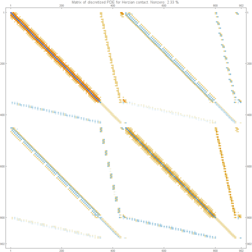
Herzian contact
The matrix of the Hertzian contact problem is shown below:

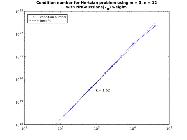
The condition number iz arther large and grows superlinearly with size in the example below.

Discussion based on practical observations
In this section we analyse different solvers, all available as part of the Eigen library supported by the Medusa. Namely we analyse the performance of two direct solvers
three combinations of general purpose iterative solver BiCGSTAB
- BiCGSTAB
- BiCGSTAB with ILUT preconditioner
- BiCGSTAB with ILUT preconditioner and exploited solveWithGuess() functionality
and a wrapper to external direct solver
The performance tests are focused on the accuracy of the numerical solution, number of iterations and time required to solve the final sparse system. We also comment on the amount of RAM required by a specific solver. If required, the gitlab repository with the implementation is also provided.
NOTE: Although the SparseQR has been included in our tests, significantly larger solve times compared to other solvers have been observed. For that reason, the SparseQR is discarded from further analyses even though it was able to obtain a solution of comparable accuracy.The two-dimensional Poisson problem
First, we solve the Poisson problem $$\nabla ^2 u(\boldsymbol x) = f(\boldsymbol x),$$
for $\boldsymbol x \in \Omega $ where the domain $\Omega$ is a unit $d=2$ dimensional circle with radius $R=1$. We use mixed boundary conditions, i.e., Dirichlet boundary for all $x < 0$ and Neumann boundary for all $x \geq 0$. Additionally, ghost or fictitious nodes were added to the Neumann boundary.
We perform analyses on two scenarios, i.e., two definitions of $f(\boldsymbol x)$:
- $f(\boldsymbol x) = -d\pi ^2 \prod_{i = 1}^d \sin(\pi x_i)$ yielding
- $f_d(\boldsymbol x) = \prod_{i = 1}^d \sin(\pi x_i)$ on the Dirichlet boundary and
- $ \boldsymbol f_n(\boldsymbol x) = \pi \sum_{i = 1}^d \cos(\pi x_i) \prod_{j=1, j\neq i}^d \sin (\pi x_j) \boldsymbol e_i$ with unit vectors $\boldsymbol e_i$ on the Neumann boundary.
- $f(\boldsymbol x) = 2a e^{-a \left \| \boldsymbol x - \boldsymbol x_s \right \|^2}(2a\left \| \boldsymbol x -
\boldsymbol x_s \right \| - d)$ yielding
- $f_d(\boldsymbol x) = e^{-a \left \| \boldsymbol x - \boldsymbol x_s \right \|^2}$ yielding on Dirichlet boundary and
- $\boldsymbol f_n (\boldsymbol x) = -2a(\boldsymbol x - \boldsymbol x_s)e^{-a \left \| \boldsymbol x - \boldsymbol x_s \right \|^2}$ on Neumann boundary.
for width $a=10^2$ of the exponential source positioned at $\boldsymbol x_s=\boldsymbol 0$.
Example solutions to both scenarios are shown in figure below.

Solver performance
Below, we show the performance of the selected solvers in case of a two-dimensional Poisson problem. The first column shows the accuracy of the numerical solution in terms of the infinity norm, the second column shows the number of iterations a given solver required (direct solvers were assigned a value 1) and the third column shows the total time required to solve the system and obtain the numerical solution $\widehat u$.
Computational times: To obtain the computational times the code was run on a single CPU with assured CPU affinity using the ''taskset'' command.

In terms of accuracy, all solvers under consideration perform equally good, with an exception of BiCGSTAB with ILUT preconditioner, who failed to obtain a solution of sufficient accuracy at the finest domain discretization with approximately $2\cdot 10^6$ nodes. The reason is most likely in the ILUT preconditioner, set to limit solver iterations to 200 with fill factor 40, drop tolerance $10^{-5}$ and global tolerance $10^{-15}$. A different ILUT setup would most probably yield a more desirable behaviour, but it nevertheless shows that when using a ILUT preconditioner one must be careful before making conclusions. It is also important to note that the SparseLU ran out of the available 11.5 Gb RAM and, therefore, failed to obtain a numerical solution. Other solvers had no issues with the available RAM space.
It is perhaps more interesting to study the number of iterations required by the solvers. Obviously, direct solvers require a "single iteration". Iterative solvers, on the other hand, require multiple iterations. Generally speaking, we observe that the number of solver iterations increases with the number of discretization points. However, it is interesting to see that the pure BiCGSTAB shows the most stable and predictable behaviour. Despite the fact that the guess provided to the BiCGSTAB is in fact the analytical solution to the problem, we do not observe significantly lower number of solver iterations.
Nevertheless, from a practical point of view, solve time is more important than the number of iterations required to obtain a numerical solution. The last column of the above figures clearly shows that the two direct solvers significantly outperform the iterative BiCGSTAB solver. On the other hand, employing BiCGSTAB with a ILUT preconditioner or providing guess to it, seems to have marginal effect on the required time.
The three-dimensional Poisson problem
Next, we test the solvers on a three-dimensional Poisson problem. The governing problem is exactly the same as in the previous case, except that the domain is a $d=3$ dimensional unit sphere.
Solver performance
Below, we show the performance of the selected solvers in case of a two-dimensional Poisson problem. The first column shows the accuracy of the numerical solution in terms of the infinity norm, the second column shows the number of iterations a given solver required (direct solvers were assigned a value 1) and the third column shows the total time required to solve the system and obtain the numerical solution $\widehat u$.


In terms of accuracy, we again observe some unexpected behaviour when ILUT preconditioner is used. This time, the ILUT preconditioner was used to limit the solver iterations to 300 with fill factor 40, drop tolerance $10^{-5}$ and global tolerance $10^{-15}$. Although 100 more iterations were allowed than in the previous two-dimensional case, this clearly was not enough for the finest domain discretizations. Additionally, providing BiCGSTAB with the analytical guess yields even more confusing results as it yielded a sudden improve of the solution accuracy. This is, of course, wrong. It is important to note that we provide analytical solution as the guess. Therefore, as soon as the solver hits the maximum allowed iterations threshold it returns the best solution currently available - largely consisting out of the analytical guess provided.
In fact, the most reliable results are again yielded by the pure BiCGSTAB and the two direct solvers. However, the two direct solvers both ran out of the available 11.5 Gb RAM space available. The SparseLU was still able to obtain a solution with $10^5$ discretization nodes, while PardisoLU seems to be more efficient since it was still able to obtain a solution with $4\cdot 10^5$ discretization points.
From the time perspective, it is clear that the two direct solvers were again significantly faster than the iterative solver - that is, of course, until they ran out of RAM. We did not come across any RAM related issues with the BiCGSTAB, even when the domain was discretized with more than a million nodes.
The linear elasticity: Boussinesq's problem
As a final problem we solve the three-dimensional Boussinesq's problem, where a concentrated normal traction acts on an isotropic half-space [1]. The same problem has also just recently been solved by employing $h$-adaptive solution procedure [2], to demonstrate the performance of a hybrid mesh-free approximation method[3] also to test the performance of $hp$-adaptive solution procedures [4].
The problem has a closed form solution given in cylindrical coordinates $r$, $\theta$ and $z$ as
$$u_r = \frac{Pr}{4\pi \mu} \left(\frac{z}{R^3} - \frac{1-2\nu}{R(z+R)} \right), \qquad u_\theta = 0, \qquad u_z = \frac{P}{4\pi \mu} \left(\frac{2(1-\nu)}{R} + \frac{z^2}{R^3} \right)$$
with stress tensor components
$$ \sigma_{rr} = \frac{P}{2\pi} \left( \frac{1-2\nu}{R(z+R)} - \frac{3r^2z}{R^5} \right), \qquad \sigma_{\theta\theta} = \frac{P(1-2\nu)}{2\pi} \left( \frac{z}{R^3} - \frac{1}{R(z+R)} \right), \qquad \sigma_{zz} = -\frac{3Pz^3}{2 \pi R^5},$$
$$ \sigma_{rz} = -\frac{3Prz^2}{2 \pi R^5} , \quad \sigma_{r\theta} = 0 , \qquad\sigma_{\theta z} = 0$$
where $P$ is the magnitude of the concentrated force, $\nu$ is the Poisson's ratio, $\mu$ is the Lame parameter and $R$ is the Eucledian distance to the origin. The solution has a singularity at the origin, which makes the problem ideal for treatment with adaptive procedures. Furthermore, the closed form solution also allows us to evaluate the accuracy of the numerical solution.
In our setup, we consider only a small part of the problem, i.e., $\varepsilon = 0.1$ away from the singularity, as schematically shown in figure below. From a numerical point of view, we solve the Navier-Cauchy Equation with Dirichlet boundary conditions described in the sketch, where the domain $\Omega$ is defined as a box, i.e., $\Omega = [-1, -\varepsilon] \times [-1, -\varepsilon] \times [-1, -\varepsilon]$.

Example solution with approximately $2\cdot 10^5$ nodes is shown below.

Solver performance
Below, we show the performance of the selected solvers in case of a three-dimensional Boussinesq's problem. The first column shows the accuracy of the numerical solution in terms of the infinity norm, the second column shows the number of iterations a given solver required (direct solvers were assigned a value 1) and the third column shows the total time required to solve the system and obtain the numerical solution $\widehat u$.

Similarly to previous studies on Poisson problems, we observe that in terms of accuracy of the numerical solution, all chosen solvers are in good agreement. However, this time we observe some desirable effects of the ILUT and guess on the performance of BiCGSTAB. Using ILUT preconditioner (and) guess reduces the number of iterations required - however, this does not notably improve the times required to obtain a numerical solution. Therefore, considering the fact that a badly-thought-out preconditioner orguess definition can notably affect the solver's performance, one is probably safer using the general purpose BiCGSTAB without the guess and without the preconditioner.
The two direct solvers were again able to solve the linear sparse system notably faster than the iterative BiCGSTAB. Unfortunately, using direct solvers we again ran into RAM space related issues.
Further literature
To read more about the solvers, we propose:
- Slovenian script by Bor Plestenjak
- Matrix Algorithms: Volume II: Eigensystems[5]
- Matrix algorithms: volume 1: basic decompositions[6]
References
- ↑ Slaughter, William S. The linearized theory of elasticity. Springer Science & Business Media, 2012.
- ↑ J. Slak and G. Kosec, Adaptive radial basis function-generated finite differences method for contact problems, International Journal for Numerical Methods in Engineering, 2019. DOI: 10.1002/nme.6067.
- ↑ M. Jančič and G. Kosec, "A hybrid RBF-FD and WLS mesh-free strong-form approximation method," 2022 7th International Conference on Smart and Sustainable Technologies (SpliTech), 2022, pp. 1-6, doi: 10.23919/SpliTech55088.2022.9854278.
- ↑ Jančič, Mitja, and Gregor Kosec. "Strong form mesh-free $ hp $-adaptive solution of linear elasticity problem." arXiv preprint arXiv:2210.07073 (2022).
- ↑ Stewart, Gilbert W. Matrix Algorithms: Volume II: Eigensystems. Society for Industrial and Applied Mathematics, 2001.
- ↑ Stewart, Gilbert W. Matrix algorithms: volume 1: basic decompositions. Society for Industrial and Applied Mathematics, 1998.