Difference between revisions of "Heat equation"
| Line 59: | Line 59: | ||
[[File:different_sigma_3.png|800px]] | [[File:different_sigma_3.png|800px]] | ||
| − | + | Graphs aren't identical. This is probably due to a slightly different domain. This happens because domain is generated with a bit of randomness. | |
We can see is that value of sigma has a big effect on relative error. | We can see is that value of sigma has a big effect on relative error. | ||
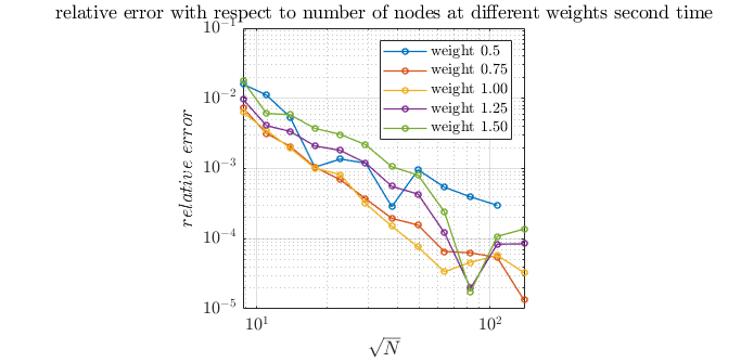
| − | Weight | + | Weight has simmilar effect on simulation as well. |
| + | |||
| + | [[File:different_weights_1.png|800px]] | ||
| + | [[File:different_weights_2.png|800px]] | ||
| + | |||
==Heat transfer== | ==Heat transfer== | ||
Revision as of 11:22, 17 September 2019
Go back to Examples.
This example shows how explicit method of solving partial differential equations is used within the Medusa library. Firstly, this example compares explicit solutions to analytical, then it shows how it can be used to solve heat transfer equation.
Contents
Domain
In this example, a square domain with a cut-out hole in the middle is used. The hole has radius equal to 1/3 of length of a square. Domain nodes are placed randomly with about dx length distance between them. Domain boundary is separated in to 5 areas: up, down, left, right and center. The idea is to have Dirichlet boundary condition on the square (up, down, left and right) and Neumann boundary conditions in the middle (center).
Fuction
The function used for this example is $u(x,y) = \sin(\pi x)\sin(\pi y)$. Laplace operator of this function is $\Delta u(x,y)=-2\pi^2\sin(\pi x)\sin(\pi y)$. For comparing explicit solution to analytical, we solve function for each node and save solution to $u\_analytic$. With this we also calculate Dirichlet boundary conditions. Then we set domain interior and nodes with Neumann bondary conditions to arbitrary value, in this case 0. We proceed to explicitly solve the domain. In the domain interior we are solving the following equation\[ \begin{align*} u (x,y,t+1) = dt*\bigg(\Delta u(x,y,t) + 2\pi^2\sin(\pi x)\sin(\pi y)\bigg)+u(x,y,t) \end{align*} \]
For Neumann bondary conditions we set $u(x,y,t+1)$ in a way that it satisfies the following equation\[ \frac{\partial u(x,y,t+1)}{\partial n}=n_x \pi \cos(\pi x) \sin(\pi y)+n_y \pi \sin(\pi x) \cos(\pi y) \]
After the simulation is finished, we can easily calculate relative error. Values of nodes are saved in a vector $u1$, so we can use norm of $|u1 - u\_analytic|$ to calculate error, then divide it by norm of $u1$ to calculate relative error.
\(
\begin{align*}
relative\_error = \frac{\sqrt{\sum{|u1-u\_analytic|^2}}}{\sqrt{\sum{|u1|^2}}}
\end{align*}
\)
Weighted Least Squares (WLS)
In this simulation, we use Gaussians for our WLS. Because of scattred nodes in our domain, we have to use 9 basis. The support size we chose is 27. For weight we have chosen 1.0 and for Gaussian weight (sigma) 75. Later we will look how change of sigma and weight effects relative error.
1 WLS<Gaussians<Vec2d>, GaussianWeight<Vec2d>, ScaleToClosest> wls({9, 75.0}, 1.0);
Finding steady state
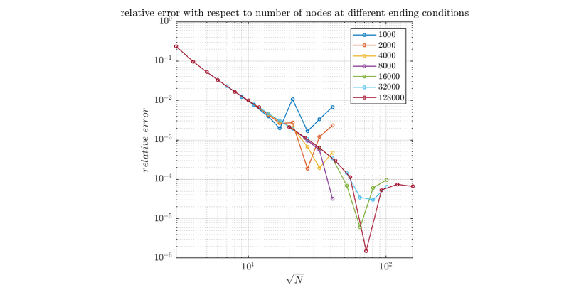
To finish simulation we save values of nodes and compare them after some time steps. Next graph shows us how relative error changes, when we increase number of steps, after which we compare values.
In this graph we can see, that using 8000 time steps is sufficient for the size of our domain, which we will use in further simulations.
Effect of sigma and weight
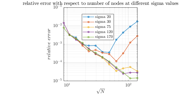
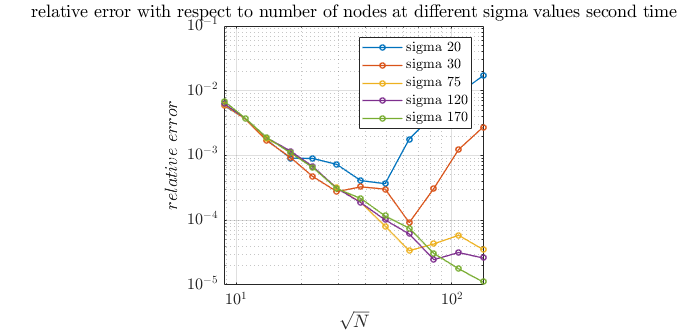
To see the effect of sigma, we ran the same simulation twice and got following graphs:
Graphs aren't identical. This is probably due to a slightly different domain. This happens because domain is generated with a bit of randomness.
We can see is that value of sigma has a big effect on relative error.
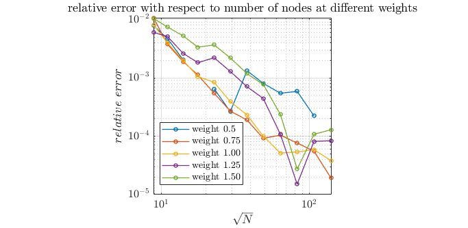
Weight has simmilar effect on simulation as well.
Heat transfer
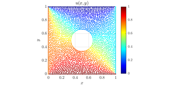
Now we use sigma 75 and weight 1.0 to solve heat transfer problem. In this case, we don't have analytical sollution. For our boundary condition, we will set up to 0.0, down to 1.0, right to 0.35 and left to 0.75. For the center hole we will use Neumann boundary conditions. We are solving following equations\[ \begin{align*} \frac{\partial u (x,y,t)}{\partial t} = \Delta u(x,y,t) \end{align*} \]
For the domain interior and for domain center we use\[ \begin{align*} \frac{\partial u (x,y,t)}{\partial n} = 0 \end{align*} \]
We get the following picture.
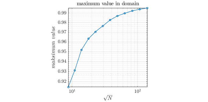
We can expect this to have the same error as the simulation with previous function. We can evaluate this by checking what the maximum value is within the domain. Doing so at different numbers of nodes gives us next graph.
Maximum value does't exceed 1.0.
Go back to Examples.
