Difference between revisions of "Schrödinger equation"
| Line 13: | Line 13: | ||
\] | \] | ||
| − | With this potential | + | With this potential Schrödinger equation simplifies to |
\[ | \[ | ||
-{\hbar^2 \over 2m} \nabla^2 \Psi(x,y,t) = i\hbar {\partial \over \partial t}\Psi(x,y,t), | -{\hbar^2 \over 2m} \nabla^2 \Psi(x,y,t) = i\hbar {\partial \over \partial t}\Psi(x,y,t), | ||
| Line 27: | Line 27: | ||
\Psi = 0 \quad \text{on} \quad \partial \Omega, | \Psi = 0 \quad \text{on} \quad \partial \Omega, | ||
\] | \] | ||
| − | where $\Omega=[0, 1]\times[0, 1]$ denotes the square box domain and $\partial \Omega$ is the boundary of the domain. In order to get the unique solution for the time propagation of the wave function the initial state $\Psi(x, y,t= 0)$ has to be selected. We choose | + | where $\Omega=[0, 1]\times[0, 1]$ denotes the square box domain and $\partial \Omega$ is the boundary of the domain. In order to get the unique solution for the time propagation of the wave function, the initial state $\Psi(x, y,t= 0)$ has to be selected. We choose |
\[ | \[ | ||
\Psi(x,y,t=0) = \sin{(\pi x)} \sin{(\pi y)}. | \Psi(x,y,t=0) = \sin{(\pi x)} \sin{(\pi y)}. | ||
\] | \] | ||
| − | Once we prepare the domain and operators, we can turn the | + | Once we prepare the domain and operators, we can turn the Schrödinger equation into code. As we are solving the time propagation implicitly, we will have to solve a matrix equation for every step. For this reason a space matrix $M$ is constructed. Next the equations are implemented, $psi$ denotes the matrix solution for each step and $rhs$ the right-hand side of the matrix equation, which is in our case equivalent to the previous state $psi$. |
| − | <syntaxhighlight lang=" | + | <syntaxhighlight lang="cpp"> |
| − | + | SparseMatrix<complex<double>, RowMajor> M(N, N); | |
| − | // | + | // Set initial state. |
for(int i : domain.interior()) { | for(int i : domain.interior()) { | ||
double x = domain.pos(i, 0); | double x = domain.pos(i, 0); | ||
| Line 44: | Line 44: | ||
} | } | ||
| − | // | + | // Set equation on interior. |
for(int i : domain.interior()) { | for(int i : domain.interior()) { | ||
| − | op.value(i) + (-1. | + | op.value(i) + (-1.0_i) * dt * op.lap(i) = rhs(i); |
} | } | ||
| − | // | + | // Set equation on boundary. |
for (int i: domain.boundary()){ | for (int i: domain.boundary()){ | ||
op.value(i) = 0; | op.value(i) = 0; | ||
| Line 55: | Line 55: | ||
</syntaxhighlight> | </syntaxhighlight> | ||
| − | At each time step the matrix equation is solved using an Eigen linear equation solver, in this case | + | At each time step the matrix equation is solved using an Eigen linear equation solver, in this case the BICGStab algorithm, and $rhs$ is updated. |
| − | <syntaxhighlight lang=" | + | <syntaxhighlight lang="cpp"> |
| − | // | + | // Solve matrix system. |
psi = solver.solve(rhs); | psi = solver.solve(rhs); | ||
| − | // | + | // Update rhs. |
rhs = psi; | rhs = psi; | ||
</syntaxhighlight> | </syntaxhighlight> | ||
| − | Time propagation of the real part of the solution $\Psi(x,y | + | Time propagation of the real part of the solution $\Psi(x,y,t)$ from times 0 to $T=0.63$ is presented below. Time step used was $10^{-5}$. |
[[File:video (1).mp4|400px]] | [[File:video (1).mp4|400px]] | ||
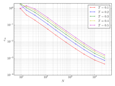
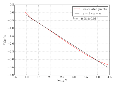
| − | As analytical solutions for infinite potential well are known this enables comparison between analytical and numerical solution computed with Medusa. On the graph bellow the error of the numerical solution is presented as maximal absolute error, meaning the largest absolute difference between numeric and its analytical solution in node at specific time. Expected linear convergence of error on a log - log scale can be observed. | + | As analytical solutions for infinite potential well are known this enables comparison between analytical and numerical solution computed with Medusa. On the graph bellow the error of the numerical solution is presented as maximal absolute error $e_{\infty}$, meaning the largest absolute difference between numeric and its analytical solution in node at specific time. Expected linear convergence of error on a log - log scale can be observed. |
| − | [[File: | + | [[File:infinite_well_2D_error.png|400px]] |
| − | [[File: | + | [[File:infinite_well_2D_error_fit.png|400px]] |
Go back to [[Medusa#Examples|Examples]]. | Go back to [[Medusa#Examples|Examples]]. | ||
Revision as of 15:17, 15 July 2019
Go back to Examples.
2D infinite square well
We are solving a Schrödinger equation for a quantum particle that is confined to a 2-dimensional square box, $0<x<L$ and $0<y<L$. Within this square the particle behaves as a free particle, but the walls are impenetrable, so the wave function is zero at the walls. This is described by the infinite potential
\[ V(x)= \begin{cases} 0, &0<x<L,\: 0<y<L, \\ \infty, &{\text{otherwise.}} \end{cases} \]
With this potential Schrödinger equation simplifies to \[ -{\hbar^2 \over 2m} \nabla^2 \Psi(x,y,t) = i\hbar {\partial \over \partial t}\Psi(x,y,t), \] where $m$ is the mass of the particle, $\hbar$ is reduced Planck constant and $\Psi(x,y,t)$ is the wave function. We set $\hbar / 2m = 1$ and $L=1$.
The solution $\Psi(x,y,t)$ must therefore satisfy \[ \nabla^2 \Psi = -i{\partial \over \partial t}\Psi \quad \text{in} \quad \Omega, \] with Dirichlet boundary condition \[ \Psi = 0 \quad \text{on} \quad \partial \Omega, \] where $\Omega=[0, 1]\times[0, 1]$ denotes the square box domain and $\partial \Omega$ is the boundary of the domain. In order to get the unique solution for the time propagation of the wave function, the initial state $\Psi(x, y,t= 0)$ has to be selected. We choose \[ \Psi(x,y,t=0) = \sin{(\pi x)} \sin{(\pi y)}. \]
Once we prepare the domain and operators, we can turn the Schrödinger equation into code. As we are solving the time propagation implicitly, we will have to solve a matrix equation for every step. For this reason a space matrix $M$ is constructed. Next the equations are implemented, $psi$ denotes the matrix solution for each step and $rhs$ the right-hand side of the matrix equation, which is in our case equivalent to the previous state $psi$.
SparseMatrix<complex<double>, RowMajor> M(N, N);

// Set initial state.
for(int i : domain.interior()) {
    double x = domain.pos(i, 0);
    double y = domain.pos(i, 1);
    rhs(i) = sin(PI * x) * sin(PI * y);
}

// Set equation on interior.
for(int i : domain.interior()) {
    op.value(i) + (-1.0_i) * dt * op.lap(i) = rhs(i);
}

// Set equation on boundary.
for (int i: domain.boundary()){
    op.value(i) = 0;
}
At each time step the matrix equation is solved using an Eigen linear equation solver, in this case the BICGStab algorithm, and $rhs$ is updated.
// Solve matrix system.
psi = solver.solve(rhs);

// Update rhs.
rhs = psi;
Time propagation of the real part of the solution $\Psi(x,y,t)$ from times 0 to $T=0.63$ is presented below. Time step used was $10^{-5}$.
As analytical solutions for infinite potential well are known this enables comparison between analytical and numerical solution computed with Medusa. On the graph bellow the error of the numerical solution is presented as maximal absolute error $e_{\infty}$, meaning the largest absolute difference between numeric and its analytical solution in node at specific time. Expected linear convergence of error on a log - log scale can be observed.
Go back to Examples.

