Difference between revisions of "Linear elasticity"
(→Cantilever beam) |
|||
| Line 9: | Line 9: | ||
== Cantilever beam == | == Cantilever beam == | ||
| − | |||
| − | |||
| − | |||
| − | |||
Consider a beam of dimensions $L \times D$ having a narrow rectangular cross section. The beam occupies a region of $[0, L] \times [-D/2, D/2]$. The beam is bent by a force $P$ applied at the end $x = 0$ and the other end of the beam is fixed at $x = L$, as illustrated below. | Consider a beam of dimensions $L \times D$ having a narrow rectangular cross section. The beam occupies a region of $[0, L] \times [-D/2, D/2]$. The beam is bent by a force $P$ applied at the end $x = 0$ and the other end of the beam is fixed at $x = L$, as illustrated below. | ||
| Line 31: | Line 27: | ||
u_y(x,y) = v(x, y) &= \frac{P}{6EI}\left(3\nu x y^2 + x^3 - 3L^2 x + 2L^3\right) | u_y(x,y) = v(x, y) &= \frac{P}{6EI}\left(3\nu x y^2 + x^3 - 3L^2 x + 2L^3\right) | ||
\end{align} | \end{align} | ||
| − | where $E$ is Young's modulus and $\nu$ is the Poisson ratio. | + | where $E$ is Young's modulus and $\nu$ is the Poisson ratio. More details can be found in [[File:Cantilever_beam.nb]]. |
The solution of the cantilever beam problem is illustrated in the <code>cantilever_beam.cpp</code> file. The problem is defined by the following pyhsical parameters: | The solution of the cantilever beam problem is illustrated in the <code>cantilever_beam.cpp</code> file. The problem is defined by the following pyhsical parameters: | ||
Revision as of 10:51, 22 January 2019
On this page we showcase some basic examples from linear elasticity. To read more about the governing equations, refer to the Solid Mechanics page
and examples therein, which are considered in more detail.
All examples here will be the solutions of the Cauchy-Navier equation $$ (\lambda + \mu) \nabla(\nabla \cdot \vec{u}) + \mu \nabla^2 \vec{u} = 0. $$
Cantilever beam
Consider a beam of dimensions $L \times D$ having a narrow rectangular cross section. The beam occupies a region of $[0, L] \times [-D/2, D/2]$. The beam is bent by a force $P$ applied at the end $x = 0$ and the other end of the beam is fixed at $x = L$, as illustrated below.
The stresses in such a beam are given as: \begin{equation} \sigma_{xx} = -\frac{Pxy}{I}, \sigma_{yy} = 0, \sigma_{xy} = -\frac{P}{2I}\left(\frac{D^2}{4} - y^2 \right), \label{eq:sxy} \end{equation} where $I = D^3/12$ is the moment of inertia.
The exact solution in terms of the displacements in $x$ and $y$ direction is \begin{align}\label{eq:beam_a1} u_x(x,y) = u(x, y) &= -\frac{Py}{6EI}\left(3(x^2-L^2) -(2+\nu)y^2 + 6 (1+\nu) \frac{D^2}{4}\right) \\ \label{eq:beam_a2} u_y(x,y) = v(x, y) &= \frac{P}{6EI}\left(3\nu x y^2 + x^3 - 3L^2 x + 2L^3\right) \end{align} where $E$ is Young's modulus and $\nu$ is the Poisson ratio. More details can be found in File:Cantilever beam.nb.
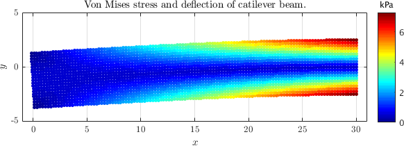
The solution of the cantilever beam problem is illustrated in the cantilever_beam.cpp file. The problem is defined by the following pyhsical parameters:
    const double E = 72.1e9;
    const double nu = 0.33;
    const double P = 1000;
    const double D = 5;
    const double L = 30;
and the problem itself is specified as follows:
    for (int i : domain.interior()) {
        (lam+mu)*op.graddiv(i) + mu*op.lap(i) = 0.0;
    }
    for (int i : domain.types() == RIGHT) {
        double y = domain.pos(i, 1);
        op.value(i) = {(P*y*(3*D*D*(1+nu) - 4*(2+nu)*y*y)) / (24.*E*I), -(L*nu*P*y*y) / (2.*E*I)};
    }
    for (int i : domain.types() == LEFT) {
        double y = domain.pos(i, 1);
        op.traction(i, lam, mu, {-1, 0}) = {0, -P*(D*D - 4*y*y) / (8.*I)};
    }
    for (int i : domain.types() == TOP) {
        op.traction(i, lam, mu, {0, 1}) = 0.0;
    }
    for (int i : domain.types() == BOTTOM) {
        op.traction(i, lam, mu, {0, -1}) = 0.0;
    }
The plot of the numerical solution produced by the accompanying cantilever_beam.m is shown below.

