Difference between revisions of "Heat equation"
(→Effect of sigma and weight) |
E6WikiAdmin (talk | contribs) |
||
| (5 intermediate revisions by 2 users not shown) | |||
| Line 42: | Line 42: | ||
WLS<Gaussians<Vec2d>, GaussianWeight<Vec2d>, ScaleToClosest> wls({9, 75.0}, 1.0); | WLS<Gaussians<Vec2d>, GaussianWeight<Vec2d>, ScaleToClosest> wls({9, 75.0}, 1.0); | ||
</syntaxhighlight> | </syntaxhighlight> | ||
| − | |||
==Effect of sigma and weight== | ==Effect of sigma and weight== | ||
| Line 72: | Line 71: | ||
We get the following picture. | We get the following picture. | ||
| − | [[File:heat_trasfer.png| | + | [[File:heat_trasfer.png|600px]] |
| − | + | [[File:heat_trasfer_2.png|600px]] | |
| − | |||
| − | [[File:heat_trasfer_2.png| | ||
| − | |||
| − | |||
| − | |||
| − | |||
| − | |||
| − | |||
| − | |||
| − | |||
Latest revision as of 20:12, 22 October 2022
Go back to Examples.
This example shows how explicit method of solving partial differential equations is used within the Medusa library. Firstly, this example compares explicit solutions to analytical, then it shows how it can be used to solve heat transfer equation.
Domain
In this example, a square domain with a cut-out hole in the middle is used. The hole has radius equal to 1/3 of length of a square. Domain nodes are placed randomly with about dx length distance between them. Domain boundary is separated in to 5 areas: up, down, left, right and center. The idea is to have Dirichlet boundary condition on the square (up, down, left and right) and Neumann boundary conditions in the middle (center).
Fuction
The function used for this example is $u(x,y) = \sin(\pi x)\sin(\pi y)$. Laplace operator of this function is $\Delta u(x,y)=-2\pi^2\sin(\pi x)\sin(\pi y)$. For comparing explicit solution to analytical, we solve function for each node and save solution to $u\_analytic$. With this we also calculate Dirichlet boundary conditions. Then we set domain interior and nodes with Neumann bondary conditions to arbitrary value, in this case 0. We proceed to explicitly solve the domain. In the domain interior we are solving the following equation\[ \begin{align*} u (x,y,t+1) = dt*\bigg(\Delta u(x,y,t) + 2\pi^2\sin(\pi x)\sin(\pi y)\bigg)+u(x,y,t) \end{align*} \]
For Neumann bondary conditions we set $u(x,y,t+1)$ in a way that it satisfies the following equation\[ \frac{\partial u(x,y,t+1)}{\partial n}=n_x \pi \cos(\pi x) \sin(\pi y)+n_y \pi \sin(\pi x) \cos(\pi y) \]
After the simulation is finished, we can easily calculate relative error. Values of nodes are saved in a vector $u1$, so we can use norm of $|u1 - u\_analytic|$ to calculate error, then divide it by norm of $u1$ to calculate relative error.
\(
\begin{align*}
relative\_error = \frac{\sqrt{\sum{|u1-u\_analytic|^2}}}{\sqrt{\sum{|u1|^2}}}
\end{align*}
\)
Weighted Least Squares (WLS)
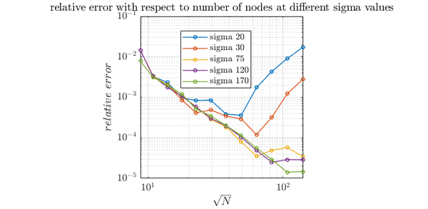
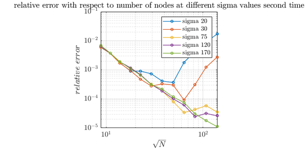
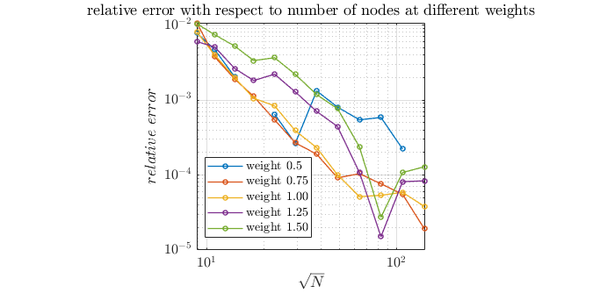
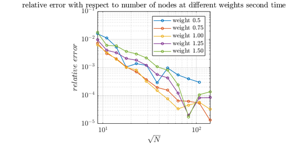
In this simulation, we use Gaussians for our WLS. Because of scattred nodes in our domain, we have to use 9 basis. The support size we chose is 27. For weight we have chosen 1.0 and for Gaussian weight (sigma) 75. Later we will look how change of sigma and weight effects relative error.
1 WLS<Gaussians<Vec2d>, GaussianWeight<Vec2d>, ScaleToClosest> wls({9, 75.0}, 1.0);
Effect of sigma and weight
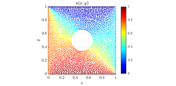
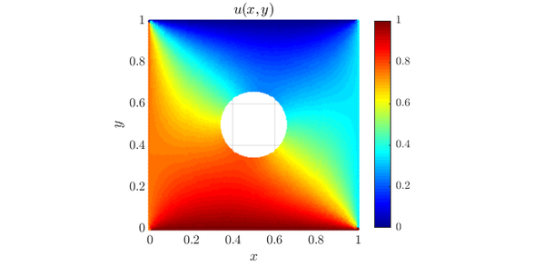
Now we use sigma 75 and weight 1.0 to solve heat transfer problem. In this case, we don't have analytical sollution. For our boundary condition, we will set up to 0.0, down to 1.0, right to 0.35 and left to 0.75. For the center hole we will use Neumann boundary conditions. We are solving following equations\[ \begin{align*} \frac{\partial u (x,y,t)}{\partial t} = \Delta u(x,y,t) \end{align*} \]
For the domain interior and for domain center we use\[ \begin{align*} \frac{\partial u (x,y,t)}{\partial n} = 0 \end{align*} \]
We get the following picture.
