Difference between revisions of "Parametric domains"
| (One intermediate revision by the same user not shown) | |||
| Line 103: | Line 103: | ||
[[File:Poisson_2D.png|800px]] | [[File:Poisson_2D.png|800px]] | ||
| − | The whole example can be found as [https://gitlab.com/e62Lab/medusa parametric_domain_2D.cpp] along with the plot script that can be run by Matlab or Octave [https://gitlab.com/e62Lab/medusa parametric_domain_2D.m | + | The whole example can be found as [https://gitlab.com/e62Lab/medusa/-/blob/dev/examples/poisson_equation/parametric_domain_2D.cpp parametric_domain_2D.cpp] along with the plot script that can be run by Matlab or Octave [https://gitlab.com/e62Lab/medusa/-/blob/dev/examples/poisson_equation/parametric_domain_2D.m parametric_domain_2D.m]. |
| − | |||
| − | |||
Latest revision as of 11:26, 1 September 2020
Go back to Examples.
Medusa supports creating domains bounded by parametric curves and (hyper-)surfaces and filling them and their interiors with node distributions of arbitrary densities.
See Positioning of computational nodes for details on node positioning algorithms.
Variable node density and Dirichlet boundary conditions in 2D
With Medusa, we can also solve partial differential equations on parametric domains. Consider the solution of a simple 2D Poisson equation with Dirichlet boundary conditions: <math> \begin{align*}
   	\Delta u &= 0.5      &&\text{in } \Omega, \\
   	  u &= 0           &&\text{on } \partial \Omega,
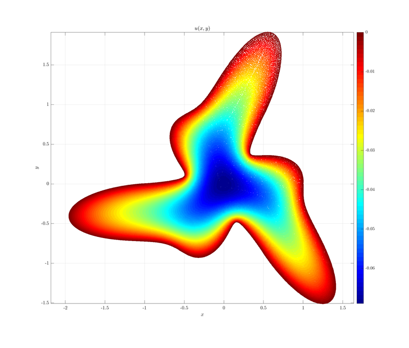
\end{align*} </math> Let's define $\Omega$ to be the interior of the parametrically given curve $r(t): [0, 2 \pi] \to \mathbb{R}^2$:
<math> \begin{align*}
   	f(t) &= |\cos(1.5 t)| ^ {\sin(3t)} \\
       r(t) &= (f(t) \cos(t), f(t) \sin(t))
\end{align*} </math> Using tools such as Wolfram Mathematica, we can find the Jacobian matrix ($\textbf{J}$) of $r$. Now, we can translate the definition of $r$ into code:
auto example_r = [](Vec<double, 1> t) {
    double r = pow(abs(cos(1.5 * t(0))), sin(3 * t(0)));
    return Vec2d(r * cos(t(0)), r * sin(t(0)));
};

auto der_example_r = [](Vec<double, 1> t) {
    double r = pow(abs(cos(1.5 * t(0))), sin(3 * t(0)));
    double der_r = (-1.5 * pow(abs(cos(1.5 * t(0))),
            sin(3 * t(0))) * sin(3 * t(0)) * sin(1.5 * t(0)) +
                    3 * pow(abs(cos(1.5 * t(0))),
                            sin(3 * t(0))) * cos(3 * t(0)) * cos(1.5 * t(0))
                            * log(abs(cos(1.5 * t(0))))) / cos(1.5 * t(0));

    Eigen::Matrix<double, 2, 1> jm;
    jm.col(0) << der_r * cos(t(0)) - r * sin(t(0)), der_r * sin(t(0)) + r * cos(t(0));

    return jm;
};

// Define parametric curve's domain.
BoxShape<Vec1d> param_bs(Vec<double, 1>{0.0}, Vec<double, 1>{2 * PI});
We implemented $r$ and $\textbf{J}$ as lambda expressions and $r$'s domain as an instance of BoxShape class. Now we can fill the target domain with nodes given by $r$ and the density function $h$ by using GeneralSurfaceFill. For the sake of this example, we choose a gradient-like density function gradient_h.
UnknownShape<Vec2d> shape;
DomainDiscretization<Vec2d> domain(shape);

auto gradient_h = [](Vec2d p){
    double h_0 = 0.005;
    double h_m = 0.03 - h_0;

    return  (0.5 * h_m * (p(0) + p(1) + 3.0) + h_0) / 5.0;
};

GeneralSurfaceFill<Vec2d, Vec1d> gsf;
domain.fill(gsf, param_bs, example_r, der_example_r, gradient_h);
After that, we can fill the interior of the domain in the usual way and choose the closest 9 nodes of each node as its support.
GeneralFill<Vec2d> gf;
domain.fill(gf, gradient_h);

int N = domain.size();
domain.findSupport(FindClosest(9));
Finally, we translate the partial differential equations of our problem into code and solve the problem, as in other examples.
int m = 2;  // basis order
Monomials<Vec2d> mon(m);
RBFFD<Polyharmonic<double, 3>, Vec2d> approx({}, mon);

// Compute the shapes (we only need the Laplacian).
auto storage = domain.computeShapes<sh::lap>(approx);

Eigen::SparseMatrix<double, Eigen::RowMajor> M(N, N);
Eigen::VectorXd rhs(N); rhs.setZero();
M.reserve(storage.supportSizes());

// Construct implicit operators over our storage.
auto op = storage.implicitOperators(M, rhs);

for (int i : domain.interior()) {
    op.lap(i) = 0.5; // set the case for nodes in the domain
}
for (int i : domain.boundary()) {
    op.value(i) = 0.0; // enforce the boundary conditions
}

Eigen::BiCGSTAB<decltype(M), Eigen::IncompleteLUT<double>> solver;
solver.compute(M);
ScalarFieldd u = solver.solve(rhs);
Here is the plot of $u(x, y)$.
The whole example can be found as parametric_domain_2D.cpp along with the plot script that can be run by Matlab or Octave parametric_domain_2D.m.
