Difference between revisions of "Analysis of MLSM performance"
(→Solving Electrostatics) |
|||
| Line 178: | Line 178: | ||
We now solve this equation for a circular enclosure with two rectangular holes. The boundary of the circular enclosure is held at constant potential $0$ V. The two rectangular holes are held at constant potentials $+1$ V and $-1$ V, respectively. A coloured scatter plot is available in figure <xr id="fig:electro_statics"/>. | We now solve this equation for a circular enclosure with two rectangular holes. The boundary of the circular enclosure is held at constant potential $0$ V. The two rectangular holes are held at constant potentials $+1$ V and $-1$ V, respectively. A coloured scatter plot is available in figure <xr id="fig:electro_statics"/>. | ||
| + | |||
| + | |||
| + | <div class="toccolours mw-collapsible mw-collapsed"> '''Code for electrostatics problem''' | ||
| + | <div class="mw-collapsible-content"> | ||
| + | |||
| + | <syntaxhighlight lang="c++" line> | ||
| + | // domain parameters, size, support and monomial order | ||
| + | int domain_size = 3000; | ||
| + | size_t n = 15; | ||
| + | size_t m = 3; | ||
| + | |||
| + | double radius = 5.0; | ||
| + | double width = 0.3; | ||
| + | double height = 3.0; | ||
| + | |||
| + | // extra boundary labels | ||
| + | int LEFT = -10; | ||
| + | int RIGHT = -20; | ||
| + | |||
| + | // build circular domain | ||
| + | CircleDomain<Vec2d> domain({0,0},radius); | ||
| + | domain.fillUniformInterior(domain_size); | ||
| + | domain.fillUniformBoundaryWithStep(domain.characteristicDistance()); | ||
| + | |||
| + | // build left rectangle | ||
| + | RectangleDomain<Vec2d> left({-2-width,-height},{-2+width,height}); | ||
| + | left.fillUniformBoundaryWithStep(domain.characteristicDistance()); | ||
| + | left.types[left.types == BOUNDARY] = LEFT; | ||
| + | domain.subtract(left); | ||
| + | |||
| + | // build right rectangle | ||
| + | RectangleDomain<Vec2d> right({2-width,-height},{2+width,height}); | ||
| + | right.fillUniformBoundaryWithStep(domain.characteristicDistance()); | ||
| + | right.types[right.types == BOUNDARY] = RIGHT; | ||
| + | domain.subtract(right); | ||
| + | |||
| + | // relax domain and find supports | ||
| + | domain.relax(50, 1e-2, 1.0, 3, 1000); | ||
| + | domain.findSupport(n); | ||
| + | |||
| + | // get interior and boundary ranges | ||
| + | Range<int> interior = domain.types == INTERNAL; | ||
| + | Range<int> boundary = domain.types == BOUNDARY; | ||
| + | Range<int> leftrect = domain.types == LEFT; | ||
| + | Range<int> rightrect = domain.types == RIGHT; | ||
| + | |||
| + | // initialize unknown concentration field and right-hand side | ||
| + | VecXd phi(domain.size(),1); | ||
| + | VecXd RHS(domain.size(),1); | ||
| + | |||
| + | // initialize interior values (this is an important step) | ||
| + | RHS[interior] = 0.0; | ||
| + | |||
| + | // set dirichlet boundary conditions | ||
| + | RHS[boundary] = 0.0; | ||
| + | RHS[leftrect] = -1.0; | ||
| + | RHS[rightrect] = 1.0; | ||
| + | |||
| + | // prepare shape functions and laplacian | ||
| + | std::vector<Triplet<double>> l_coeff; | ||
| + | for (auto& c : interior) { | ||
| + | Range<Vec2d> supp_domain = domain.positions[domain.support[c]]; | ||
| + | EngineMLS<Vec2d, Monomials, Gaussians> MLS(m,supp_domain,pow(domain.characteristicDistance(),2)); | ||
| + | VecXd shape = MLS.getShapeAt(supp_domain[0], {{2, 0}}) + | ||
| + | MLS.getShapeAt(supp_domain[0], {{0, 2}}); | ||
| + | for (size_t i = 0; i < supp_domain.size(); ++i) { | ||
| + | l_coeff.emplace_back(c, domain.support[c][i], shape[i]); | ||
| + | } | ||
| + | } | ||
| + | |||
| + | // prepare dirichlet boundaries | ||
| + | std::vector<Triplet<double>> b_coeff; | ||
| + | for (auto& c : domain.types < 0) { | ||
| + | b_coeff.emplace_back(c, c, 1.0); | ||
| + | } | ||
| + | |||
| + | // prepare matrices | ||
| + | SparseMatrix<double> laplace_m(domain.size(), domain.size()); | ||
| + | laplace_m.setFromTriplets(l_coeff.begin(), l_coeff.end()); | ||
| + | SparseMatrix<double> boundary_m(domain.size(), domain.size()); | ||
| + | boundary_m.setFromTriplets(b_coeff.begin(), b_coeff.end()); | ||
| + | |||
| + | // draw | ||
| + | std::thread th([&] { draw2D(domain.positions, phi); }); | ||
| + | |||
| + | // initialize solver | ||
| + | Eigen::BiCGSTAB<SparseMatrix<double>> solver; | ||
| + | |||
| + | // join matrices together | ||
| + | SparseMatrix<double> tmp = boundary_m + laplace_m; | ||
| + | solver.compute(tmp); | ||
| + | |||
| + | // solve system of equations | ||
| + | phi = solver.solve(RHS); | ||
| + | std::cout << "#iterations: " << solver.iterations() << std::endl; | ||
| + | std::cout << "estimated error: " << solver.error() << std::endl; | ||
| + | |||
| + | // end drawing | ||
| + | th.join(); | ||
| + | </syntaxhighlight> | ||
| + | |||
| + | </div> | ||
| + | </div> | ||
| + | |||
<figure id="fig:electro_statics"> | <figure id="fig:electro_statics"> | ||
[[File:electro_statics.png|thumb|upright=2|center|<caption> Simple electrostatics problem solved by implicit method with 15 node monomial supports and gaussian weight functions. </caption>]] | [[File:electro_statics.png|thumb|upright=2|center|<caption> Simple electrostatics problem solved by implicit method with 15 node monomial supports and gaussian weight functions. </caption>]] | ||
</figure> | </figure> | ||
Revision as of 11:44, 28 November 2016
Contents
Solving Diffusion equation
For starters, we can solve simple Diffusion equation $ \nabla^2 u = \frac{\partial u}{\partial t} $.
We solved the equation on a square $\Omega = [0, a] \times [0, a]$ with Dirichlet boundary conditions $ \left. u\right|_{\partial \Omega} = 0 $ and initial state $ u(t = 0) = 1$.
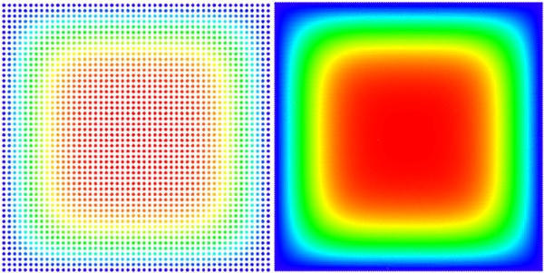
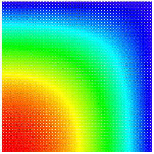
An analytical solution for this domain is known, and we use it to evaluate or own solution. \begin{equation} u(\vec{p}, t) = \sum_{\substack{n=1 \\ n \text{ odd}}}^\infty\sum_{\substack{m=1 \\ m \text{ odd}}}^\infty \frac{1}{\pi^2} \frac{16 a^2}{nm} \sin\left(\frac{\pi n}{a}p_x\right) \sin\left(\frac{\pi m}{a}p_y\right) e^{-\frac{\pi^2 (n^2+m^2)}{a^2}t} \end{equation} Because the solution is given in the series form, we only compare to the finite approximation, summing to $N = 100$ instead of infinity. Solution is on Figure 1. See the code for solving diffusion here.
Analysis of our method
Convergence with respect to number of nodes
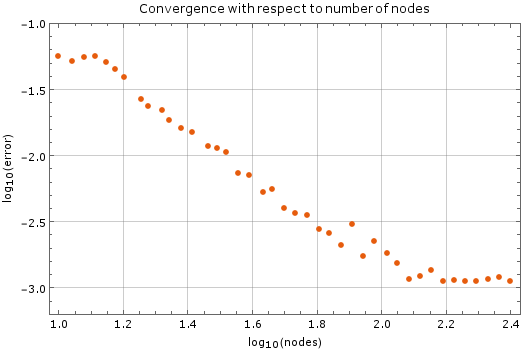
We tested the method with a fixed time step of $ \Delta t = 1\cdot 10^{-5}$ on a unit square ($a = 1$). Results are on Figure 2. Monomial basis of $6$ monomials was used and $12$ closest nodes counted as support for each node. After more than $250$ nodes of discretization in each dimension the method diverges, which is expected. The stability criterion for diffusion equation in two dimensions is $\Delta t \leq \frac{1}{4} \Delta x^2$, where $\Delta x$ is the spatial discretization step in one dimension. In our case, at $250$ nodes per side, the right hand side yields $\frac{1}{4}\cdot\frac{1}{250}\cdot\frac{1}{250} = 4\times 10^{-6}$, so our method is stable within the expected region.
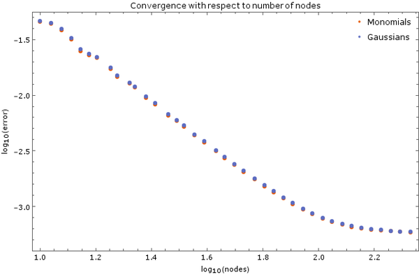
On Figure 3 is another image of convergence, this time using monomial basis $\{1, x, y, x^2, y^2\}$ and Gaussian basis with discretization step $ \Delta t = 5 \cdot 10^{-6}$ and 5 support nodes. Total node count was $N = 2500$. Error was calculated after $0.01$ time units have elapsed.
Convergence with respect to number of time steps
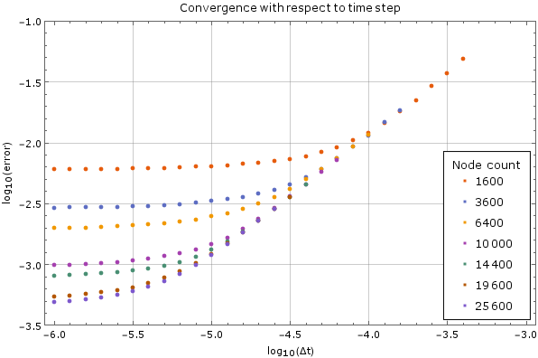
We tested the method on a fixed node count with different time steps on the same domain as above. Results are on Figure 4. For large time steps the method diverges, but once it starts converging the precision increases steadily as the time step decreases, until it hits its lower limit. This behaviour is expected. The error was calculated against the analytical solution above after $0.005$ units of time have passed. A monomial basis up to order $2$ inclusive ($m = 6$) was used and the support size was $n = 12$.
Using Gaussian basis
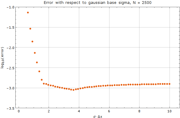
We tested the method on a fixed node count of $N = 2500$ with spatial step discretization of $\Delta x = \frac{1}{50}$. We used the Gaussian basis of $m = 5$ functions with support size $n = 13$. Error was calculated against analytical solution above after $0.01$ time units. A time step of $\Delta t = 10^{-5}$ was used. Results are on Figure 5
As we can see from the graph, there exists an interval where the choice of $\sigma$ does not matter much, but outside of this interval, the method diverges rapidly. Care from the user side must be taken, to choose $\sigma$ appropriately, with respect to plot above.
Solving in 3D
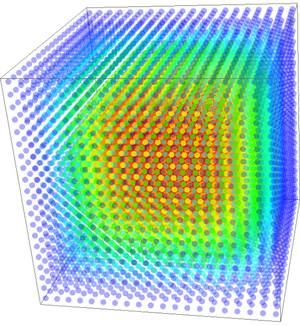
A 3-dimensional case on domain $[0, 1]^3$ was tested on $N = 20^3$ nodes, making the discretization step $\Delta x = 0.05$. Support size of $n=10$ with $m=10$ Gaussian basis functions was used. Their normalization parameter was $\sigma = 60\Delta x$. A time step of $\Delta t = 10^{-5}$ and an explicit Euler method was used to calculate the solution of to $0.01$ time units. Resulting function is on Figure 6.
Solving Dirichlet with EngineMLS
Example code using explicit stepping to reproduce the thermal images from the beginning: example code
Solving Dirichlet with MLSM operators
Example code using explicit stepping and MLSM operators to reproduce the thermal images from the beginning: example code
Solving mixed boundary conditions with MLSM operators
By using MLSM operators and utilizing its `MLSM::neumann` method we can also solve partial diffusion equations. Solution is on Figure 7.
Example code showing the use of Neumann boundary conditions: example code
We also support more -- interesting -- domains :) On Figure 8 we see a domain in a shape of Miki mouse.
Convergence analysis for one dimensional diffusion equation
We now tried to solve the diffusion equation in one dimension $u_t = u_{xx}$ on the interval $[0,1]$ with Dirichlet boundary conditions $u(0, t) = u(1,t) = 0 $ and an initial state $u(x,0) = \sin(\pi x).$
An analytical solution for this domain is given in closed form \begin{equation} u(x,t) = \sin(\pi x) \exp(-\pi^2 t), \end{equation} so we can use it to evaluate our approximation.
We tested the method with a fixed time step of $\Delta t = 1\cdot 10^{-8}$ on a unit interval, that was discretized into $ N $ nodes. Monomial basis of $m$ monomials was used and $n$ closest nodes counted as support for each node.
Note: the results are not confirmed and serve merely as an orientation. Errors may have occured.
Convergence with respect to number of nodes and support size
Convergence of the method was tested on different number of nodes $N = 15, 20, 25, \ldots, 200$. First we tested the method, when support size is equal to number of monomials in the basis ($n =m$), which we call local interpolation, for different values of $n = 3, 5, 7$. We then compared that to local approximation, where we take $n = 12$ supporting nodes and we only change number of monomials. We used gaussian weight function with $\sigma = 1\cdot \Delta x$. Error was calculated after $0.001$ time units have elapsed. We can see the results on Figure 9.
Larger is the support size, faster is convergence. This rule applies for local interpolation as well as approximation. But when number of nodes is too large, the method diverges faster for larger support sizes. Error for approximation is bigger than for interpolation (if we compare it for same basis size), but the method diverges with interpolation for smaller number of nodes.
Convergence with respect to weight function
We also checked the convergence for different weight functions. We tested it on number of nodes $N = 15, 20, 25, \ldots, 200$, with monomial basis with $m = 5$, support size $n = 12$ and gaussian weight function with $\sigma = w\cdot \Delta x$ for $w = 0.1$. Error was calculated after $0.001$ time units have elapsed with $\Delta t = 10^{-8}$. We can see the results on Figure 10.
When the $\sigma$ is too small, other nodes on the support domain are not taken into consideration, so taking $n = 12$ or $n = 3$ would give the same results. However when $\sigma$ is too large, all the nodes on the support domain are contributing and there is no significant difference between different weight functions.
Solving Electrostatics
This example is taken from the FreeFem++ manual (page 235).
Assuming there is no current and the charge distribution is time independent, the electric field $\b{E}$ satisfies \begin{equation}\label{eq:electrostatics} \b{\nabla}\cdot\b{E} = \frac{\rho}{\epsilon}, \quad \b{\nabla} \times \b{E} = 0 \end{equation} where $\rho$ is the charge density and $\epsilon$ is the permittivity. If we introduce an electrostatics potential $\phi$ such that \begin{equation} \b{E} = -\b{\nabla}\phi, \end{equation} we can insert it into the first equation in (\ref{eq:electrostatics}) resulting in Poisson's equation \begin{equation}\label{eq:poisson} \b{\nabla}^2 \phi = -\frac{\rho}{\epsilon}. \end{equation} In the absence of unpaired electric charge equation (\ref{eq:poisson}) becomes Laplace's equation \begin{equation} \b{\nabla}^2 \phi = 0 \end{equation}
We now solve this equation for a circular enclosure with two rectangular holes. The boundary of the circular enclosure is held at constant potential $0$ V. The two rectangular holes are held at constant potentials $+1$ V and $-1$ V, respectively. A coloured scatter plot is available in figure Figure 11.
 1     // domain parameters, size, support and monomial order
 2     int domain_size = 3000;
 3     size_t n = 15;
 4     size_t m = 3;
 5
 6     double radius = 5.0;
 7     double width = 0.3;
 8     double height = 3.0;
 9
10     // extra boundary labels
11     int LEFT = -10;
12     int RIGHT = -20;
13
14     // build circular domain
15     CircleDomain<Vec2d> domain({0,0},radius);
16     domain.fillUniformInterior(domain_size);
17     domain.fillUniformBoundaryWithStep(domain.characteristicDistance());
18
19     // build left rectangle
20     RectangleDomain<Vec2d> left({-2-width,-height},{-2+width,height});
21     left.fillUniformBoundaryWithStep(domain.characteristicDistance());
22     left.types[left.types == BOUNDARY] = LEFT;
23     domain.subtract(left);
24
25     // build right rectangle
26     RectangleDomain<Vec2d> right({2-width,-height},{2+width,height});
27     right.fillUniformBoundaryWithStep(domain.characteristicDistance());
28     right.types[right.types == BOUNDARY] = RIGHT;
29     domain.subtract(right);
30
31     // relax domain and find supports
32     domain.relax(50, 1e-2, 1.0, 3, 1000);
33     domain.findSupport(n);
34
35     // get interior and boundary ranges
36     Range<int> interior = domain.types == INTERNAL;
37     Range<int> boundary = domain.types == BOUNDARY;
38     Range<int> leftrect = domain.types == LEFT;
39     Range<int> rightrect = domain.types == RIGHT;
40
41     // initialize unknown concentration field and right-hand side
42     VecXd phi(domain.size(),1);
43     VecXd RHS(domain.size(),1);
44
45     // initialize interior values (this is an important step)
46     RHS[interior] = 0.0;
47
48     // set dirichlet boundary conditions
49     RHS[boundary] = 0.0;
50     RHS[leftrect] = -1.0;
51     RHS[rightrect] = 1.0;
52
53     // prepare shape functions and laplacian
54     std::vector<Triplet<double>> l_coeff;
55     for (auto& c : interior) {
56         Range<Vec2d> supp_domain = domain.positions[domain.support[c]];
57         EngineMLS<Vec2d, Monomials, Gaussians> MLS(m,supp_domain,pow(domain.characteristicDistance(),2));
58         VecXd shape = MLS.getShapeAt(supp_domain[0], {{2, 0}}) +
59                       MLS.getShapeAt(supp_domain[0], {{0, 2}});
60         for (size_t i = 0; i < supp_domain.size(); ++i) {
61             l_coeff.emplace_back(c, domain.support[c][i], shape[i]);
62         }
63     }
64
65     // prepare dirichlet boundaries
66     std::vector<Triplet<double>> b_coeff;
67     for (auto& c : domain.types < 0) {
68         b_coeff.emplace_back(c, c, 1.0);
69     }
70
71     // prepare matrices
72     SparseMatrix<double> laplace_m(domain.size(), domain.size());
73     laplace_m.setFromTriplets(l_coeff.begin(), l_coeff.end());
74     SparseMatrix<double> boundary_m(domain.size(), domain.size());
75     boundary_m.setFromTriplets(b_coeff.begin(), b_coeff.end());
76
77     // draw
78     std::thread th([&] { draw2D(domain.positions, phi); });
79
80     // initialize solver
81     Eigen::BiCGSTAB<SparseMatrix<double>> solver;
82
83     // join matrices together
84     SparseMatrix<double> tmp = boundary_m + laplace_m;
85     solver.compute(tmp);
86
87     // solve system of equations
88     phi = solver.solve(RHS);
89     std::cout << "#iterations:     " << solver.iterations() << std::endl;
90     std::cout << "estimated error: " << solver.error()      << std::endl;
91
92     // end drawing
93     th.join();
