Revision as of 11:31, 15 November 2016 (view source) Ipribec (talk | contribs) (→‎References) ← Older edit		Revision as of 11:37, 15 November 2016 (view source) Ipribec (talk | contribs) (→‎Exact solution) Newer edit →
Line 5:		Line 5:
	= Exact solution =		= Exact solution =
−	The exact solutions to this problem is given in Timoshenko (1951) where it derived for '''plane stress''' conditions. Consider a beam of dimensions $L \times D$ having a narrow rectangular cross section. The origin of the coordinate system is placed at $(x,y) = (0,D/2)$. The beam is bent by a force $P$ applied at the end $x = 0$ and the other end of the beam is fixed (at $x = L$). The stresses in such a beam are given as:	+	The exact solutions to this problem is given by Timoshenko (1951) where it derived for '''plane stress''' conditions <ref>Timoshenko, S. and Goodier, J. N. (1951). ''Theory of elasticity'', p. 35 - 39. McGraw-Hill, Inc., New York.</ref>. Consider a beam of dimensions $L \times D$ having a narrow rectangular cross section. The origin of the coordinate system is placed at $(x,y) = (0,D/2)$. The beam is bent by a force $P$ applied at the end $x = 0$ and the other end of the beam is fixed (at $x = L$). The stresses in such a beam are given as:
	\begin{equation}		\begin{equation}
	\sigma_{xx} = -\frac{Pxy}{I},		\sigma_{xx} = -\frac{Pxy}{I},

---

Revision as of 11:37, 15 November 2016

Do you want to go back to Solid Mechanics?

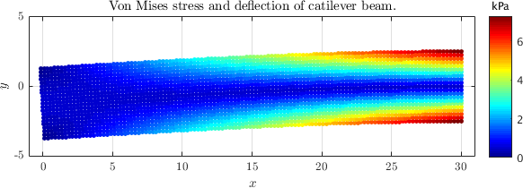
On this page we conduct numerical studies of bending of a cantilever loaded at the end, a common numerical benchmark in elastostatics.

Exact solution

The exact solutions to this problem is given by Timoshenko (1951) where it derived for plane stress conditions ^[1]. Consider a beam of dimensions $L \times D$ having a narrow rectangular cross section. The origin of the coordinate system is placed at $(x,y) = (0,D/2)$. The beam is bent by a force $P$ applied at the end $x = 0$ and the other end of the beam is fixed (at $x = L$). The stresses in such a beam are given as:

$$\begin{equation} \sigma_{xx} = -\frac{Pxy}{I}, \end{equation}$$ $$\begin{equation} \sigma_{yy} = 0, \end{equation}$$ $$\begin{equation}\label{eq:sxy} \sigma_{xy} = -\frac{P}{2I}\left(\left(\frac{D}{2}\right)^2 - y^2 \right), \end{equation}$$ where $I = D^3/12$ is the moment of inertia.

The exact solution in terms of the displacements in $x$- and $y-$ direction is

$$\begin{align}\label{eq:beam_a1} u_x(x,y) &= -\frac{Py}{6EI}\left(3(x^2-L^2) -(2+\nu)y^2 + 6 (1+\nu) \frac{D^2}{4}\right) \\ \label{eq:beam_a2} u_y(x,y) &= \frac{P}{6EI}\left(3\nu x y^2 + x^3 - 3L^2 x + 2L^3\right) \end{align}$$ where $E$ is Young's modulus and $\nu$ is the Poisson ratio.

Numerical solution

For the numerical solution we first choose the following parameters:

• Loading: $P = -1000$ N
• Young's modulus: $E = 3 \times 10^7$ N/m²
• Poisson's ratio: $\nu = 0.3$
• Height of the beam: $D = 12$ m
• Length of the beam: $L = 48$ m

The unloaded beam is discretized with $40 \times 10$ regular nodes. Since the right end of the beam at $x = L$ is fixed, the displacement boundary conditions are prescribed from the known analytical formulae ($\ref{eq:beam_a1}$) and ($\ref{eq:beam_a2}$) :

$$\begin{equation} u_x(L,y) = -\frac{P}{6EI}\left(-(2+\nu)y^2 + 6 (1+\nu) \frac{D^2}{4}\right); \qquad u_y(L,y) = \frac{P}{2EI}(\nu L y^2) \end{equation}$$ The traction boundary at the left end of the beam ($x=0$) is given by ($\ref{eq:sxy}$): $$\begin{equation}\label{eq:trac_a} t_y(L,y) = -\frac{P}{2I}\left(\left(\frac{D}{2}\right)^2 - y^2 \right). \end{equation}$$

An indicator of the accuracy that can be employed is the strain energy error $e$:

$$\begin{equation} e = \left[ \frac{1}{2} \int_\Omega (\b{\varepsilon}^\mathrm{num} - \b{\varepsilon}^\mathrm{exact})\b{C}(\b{\varepsilon}^\mathrm{num} - \b{\varepsilon}^\mathrm{exact}) d\Omega\right]^{1/2} \end{equation}$$ where $\b{\varepsilon}$ is the strain tensor in vector form, $\b{C}$ the reduced stiffness tensor (a matrix) and $\Omega$ the domain of the calculated solution.

FreeFem++

The required code to solve this problem in FreeFem++ is

// Parameters
real E = 3.0e7, nu = 0.3;
real P = -1000;
real L = 48, D = 12;
real I = D^3/12;

// Mesh
mesh Th = square(40,10,[L*x,-D/2+D*y]);

// Macros
macro u [ux,uy] // displacement
macro v [vx,vy] // test function
macro div(u) (dx(u[0])+dy(u[1])) // divergence
macro eM(u) [dx(u[0]), dy(u[1]), sqrt(2)*(dx(u[1]) + dy(u[0]))/2] // strain tensor

// Finite element space
fespace Vh(Th,[P2,P2]);
Vh u, v;

// Boundary conditions
func uxb = -P*y/(6*E*I)*(nu*y^2-2*(1+nu)*y^2+6*D^2/4*(1+nu));
func uyb = P/(6*E*I)*(3*nu*L*y^2);
func ty = -P/(2*I)*(D^2/4-y^2);

// Convert E and nu to plane stress
E = E/(1-nu^2); nu = nu/(1-nu);

// Lame parameters
real mu = E/(2*(1+nu));
real lambda = E*nu/((1+nu)*(1-2*nu));

// Solve problem
solve cantileverBeam(u,v) =
   int2d(Th)(lambda*div(u)*div(v) + 2*mu*(eM(u)'*eM(v)))
   - int1d(Th,4)([0,-ty]'*v)
   + on(2,ux=uxb,uy=uyb);

// Plot solution
real coef = 1000;
Th = movemesh(Th,[x+ux*coef,y+uy*coef]);
plot(Th,wait=1);

The numerical solutions for beam displacements $u_y(x,0)$ in the axial direction of the beam, and shear stresses $\sigma_{xy}(L/2,y)$ in a cross section at the half lengthwise of the beam, obtained by quadratic finite elements are shown in the figure below. Analytic solutions are shown with continuous lines.

Reference test

This is the text that you are going to verify with a reference.^[2]

References

1. Jump up ↑ Timoshenko, S. and Goodier, J. N. (1951). Theory of elasticity, p. 35 - 39. McGraw-Hill, Inc., New York.
2. Jump up ↑ Reference details go here