Difference between revisions of "Positioning of computational nodes"
(→Relaxation of the nodal distribution) |
E6WikiAdmin (talk | contribs) |
||
| (119 intermediate revisions by 4 users not shown) | |||
| Line 1: | Line 1: | ||
| − | + | {{Box-round|title= Related papers | | |
| − | |||
| − | + | [https://e6.ijs.si/ParallelAndDistributedSystems/publications/98533123.pdf M. Depolli, J. Slak, G. Kosec; Parallel domain discretization algorithm for RBF-FD and other meshless numerical methods for solving PDEs, Computers & Structures, 2022 [DOI: 10.1016/j.compstruc.2022.106773]] | |
| − | |||
| − | + | [https://e6.ijs.si/ParallelAndDistributedSystems/publications/32782887.pdf J. Slak, G. Kosec; On generation of node distributions for meshless PDE discretizations, SIAM journal on scientific computing, vol. 41, 2019 [DOI: 10.1137/18M1231456]] | |
| − | |||
| − | |||
| − | |||
| − | |||
| − | + | [https://e6.ijs.si/ParallelAndDistributedSystems/publications/56730115.pdf U. Duh, G. Kosec, J. Slak; Fast variable density node generation on parametric surfaces with application to mesh-free methods, SIAM journal on scientific computing, vol. 43, 2021 [DOI: 10.1137/20M1325642]] | |
| − | |||
| − | |||
| − | |||
| − | |||
| − | |||
| − | |||
| − | |||
| − | |||
| − | |||
| − | |||
| − | |||
| − | |||
| − | |||
| − | |||
| − | + | [https://e6.ijs.si/ParallelAndDistributedSystems/publications/69777155.pdf J. Slak, G. Kosec; Medusa : A C++ library for solving PDEs using strong form mesh-free methods, ACM transactions on mathematical software, vol. 47, 2021 [DOI: 10.1145/3450966]] | |
| − | + | }} | |
| − | |||
| − | |||
| − | |||
| − | |||
| − | |||
| − | |||
| − | |||
| − | |||
| − | |||
| − | |||
| − | |||
| − | |||
| − | |||
| − | + | __TOC__ | |
| − | + | Since one of the most attractive features of mesh-free methods is the ability to use nodes | |
| + | without any connectivity information, node placing was considered much easier than mesh generation | ||
| + | or simply used existing tools for mesh generation and was thus often disregarded, | ||
| + | sometimes implying that any nodes could be used, even if placed at random. | ||
| + | It soon turned out that that is not the case, mostly with strong form methods, | ||
| + | since many methods require regular nodes for good performance and bad distributions | ||
| + | can impact their stability. | ||
| − | == | + | |
| − | To | + | One of the key successes of RBF based mesh free methods, such as RBF-generated finite differences |
| + | (RBF-FD) is the ability to use highly spatially variable node distributions which can | ||
| + | adapt to irregular geometries and allow for refinement in critical areas. | ||
| + | We present our algorithms below. Their goal is to fill an arbitrary domain $\Omega \subseteq \R^d$ with nodes following the given target spacing function $h(\b{p}): \Omega \to (0, \infty)$, which maps points from $\Omega$ to desired distance to neighboring points. | ||
| + | |||
| + | Please refer to following papers for mode details: | ||
| + | |||
| + | |||
| + | == Measures of node regularity == | ||
| + | |||
| + | To analyze the regularity of nodes locally, we find $c$ nearest neighbors $\b{p}_{i, j}, j = 1, 2, \dots c$ of each node $\b{p}_i$. Local regularity can now be measured with | ||
| + | \begin{align*} | ||
| + | \bar{d}_i = \frac{1}{c} \sum_{j =1}^{c}\|\b{p}_i - \b{p}_{i, j}\| & \quad \dots \quad \text{average distance to} \ c \ \text{nearest neighbors}, \\ | ||
| + | d_i^{\text{min}} = \min_{j=1, \dots c} \|\b{p}_i - \b{p}_{i, j}\| & \quad \dots \quad \text{minimum distance to} \ c \ \text{nearest neighbors}, \\ | ||
| + | d_i^{\text{max}} = \max_{j=1, \dots c} \|\b{p}_i - \b{p}_{i, j}\| & \quad \dots \quad \text{maximum distance to} \ c \ \text{nearest neighbors}. \\ | ||
| + | \end{align*} | ||
| + | We can also normalize the quantities by scaling them with $h$, thus getting $d'_i = d_i / h(\b{p}_i)$. It is therefore desirable that all the normalised above quantities are approximately equal to $1$. | ||
| + | |||
| + | Global regularity can be assessed by plotting distributions of local regularity measures. For example, a desirable distribution of $\bar{d}'_i$ would have maximum and average approximately equal to $1$ and a low standard deviation. If $h$ is a constant function, a discretization of $\Omega$ with point set $\mathcal{X} = {x_1, \dots, x_N} \subseteq \Omega$ can also be assessed with standard concepts such as<ref name="ScatteredData">H. Wendland, Scattered data approximation, vol. 17, Cambridge university press, 2004.</ref> | ||
| + | \begin{align*} | ||
| + | r_{\max, \mathcal{X}} = \sup_{x \in \Omega} \min_{1 \leq j \leq N} \|x - x_j\| & \quad \dots \quad \text{maximum empty sphere radius}, \\ | ||
| + | r_{\min, \mathcal{X}} = \frac{1}{2} \min_{i \neq j} \| x_i - x_j \| & \quad \dots \quad \text{separation distance}. \\ | ||
| + | \end{align*} | ||
| + | Those can also be normalized, getting $r' = r / h$. It is desirable that both $r'_\max$ and $r'_\min$ are approximately equal to $\frac{1}{2}$, however values of $r_\max$ around $2$ (especially when $N$ is small) are also considered good enough. In practice, the maximum empty sphere radius can be numerically estimated by discretizing $\Omega$ with a much smaller nodal spacing $h$ and calculating the maximum empty sphere radius with center in one of the generated nodes. | ||
| + | |||
| + | == Filling domain interior == | ||
| + | |||
| + | We start with a simple algorithm based on '''Poisson Disk Sampling''' (PDS) that results in a relatively tightly packed distribution of nodes. | ||
| + | The algorithm beings with a given non-empty set of nodes called "seed nodes". | ||
| + | A single seed node placed anywhere in the domain interior is needed to begin the | ||
| + | algorithm and if none are provided, one can be chosen at random. | ||
| + | However, in the context of PDE discretisations, some nodes on the boundary are usually | ||
| + | already known and can be used as seed nodes, possibly along with additional nodes in the interior. | ||
| + | |||
| + | The initial nodes are put in a queue. In each iteration $i$, a new node $\b{p}_i$ is dequeued. | ||
| + | Its desired nodal spacing $r_i$ is obtained from the function $h$, $r_i = h(\b{p}_i)$. A | ||
| + | set $C_i$ of $n$ new candidates is generated, which lie on the sphere with center $\b{p}_i$ and radius $r_i$. | ||
| + | New candidates are spaced uniformly with a random rotation. | ||
| + | Candidates that lie outside of the domain or are too close to already existing nodes | ||
| + | are rejected. Nearest neighbor search is performed by a spatial search structure, usually a [[K-d tree|''k''-d tree]] is used. Remaining candidates are enqueued and node $\b{p}_i$ is marked as "expanded". | ||
| + | The iteration continues until the queue is empty. | ||
| + | |||
| + | An illustration of the algorithm's progress on a unit square can be seen in <xr id="fig:gf_generation"/><ref name="GeneralFill">J. Slak and G. Kosec, On generation of node distributions for meshless PDE discretizations, SIAM Journal on Scientific Computing, 41 (2019), | ||
| + | pp. A3202–A3229, https://doi.org/10.1137/18M1231456.</ref>. | ||
| + | |||
| + | <figure id="fig:gf_generation"> | ||
| + | [[File:gf_generation.png|1000px|thumb|center|<caption> Progress of the interior filling algorithm on a unit square. </caption>]] | ||
| + | </figure> | ||
| + | |||
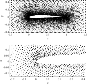
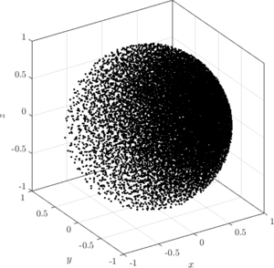
| + | See <xr id="fig:gf_examples_1"/> and <xr id="fig:gf_examples_2"/> for examples of discretized 2D and 3D domains. | ||
| + | |||
| + | <figure id="fig:gf_examples_1"> | ||
| + | [[File:2d_poisson_disk_sampling.png|thumb|<caption> Examples of 2D domains filled by the interior filling algorithm. </caption>]] | ||
| + | </figure> | ||
| + | |||
| + | <figure id="fig:gf_examples_2"> | ||
| + | [[File:3d_poisson_disk_sampling.png|thumb|<caption> Example of a 3D domain filled by the interior filling algorithm. </caption>]] | ||
| + | </figure> | ||
| + | |||
| + | The interior filling algorithm is thoroughly analyzed in <ref name="GeneralFill"/>. It is implemented in Medusa as [http://e6.ijs.si/medusa/docs/html/classmm_1_1GeneralFill.html GeneralFill]. | ||
| + | |||
| + | === Regularity analysis === | ||
| + | |||
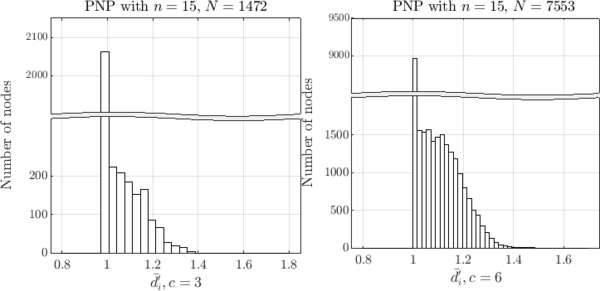
| + | See <xr id="fig:gf_hist"/><ref name="GeneralFill"/> for a distribution of normalized average distances to $c = 3$ nearest neighbors on a 2D unit square (left) and $c = 6$ nearest neighbors on a 3D unit cube (right) filled with constant $h$. The distribution is satisfactory, since it has a lower standard deviation and maximum around $1$. See also the table below for other global measures of regularity for the same cases as those on the histograms. | ||
| + | |||
| + | <figure id="fig:gf_hist"> | ||
| + | [[File:gf_hist.png|thumb|center|600px|<caption> Distribution of normalized distances to $c = 3$ nearest neighbors on a 2D unit square (left) and $c = 6$ nearest neighbors on a 3D unit cube (right) filled with constant $h$. </caption>]] | ||
| + | </figure> | ||
| + | |||
| + | {| class="wikitable" style="margin-left: auto; margin-right: auto; border: none;" | ||
| + | !colspan="6"|Measures of regularity | ||
| + | |- | ||
| + | |dim. | ||
| + | |$\text{mean} \, \bar{d}'_i$ | ||
| + | |$\text{std} \, \bar{d}'_i$ | ||
| + | |$\text{mean} \left(\left(d_i^{\text{max}}\right)' - \left(d_i^{\text{min}}\right)'\right)$ | ||
| + | |$r'_\min$ | ||
| + | |$r'_\max$ | ||
| + | |- | ||
| + | |2D | ||
| + | |$1.0416$ | ||
| + | |$0.0344$ | ||
| + | |$0.0832$ | ||
| + | |$0.5000$ | ||
| + | |$2.0656$ | ||
| + | |- | ||
| + | |3D | ||
| + | |$1.0508$ | ||
| + | |$0.0418$ | ||
| + | |$0.0849$ | ||
| + | |$0.5000$ | ||
| + | |$2.1023$ | ||
| + | |} | ||
| + | |||
| + | === Computational complexity === | ||
| + | |||
| + | Computational complexity of the interior filling algorithm is<ref name="GeneralFill"/> | ||
| + | \begin{equation} | ||
| + | T_{\text{interior}} = O(P(N) + NnQ(N)+NI(N)), | ||
| + | \end{equation} | ||
| + | where $N$ is the number of generated nodes, $P$ is the precomputation complexity of the spatial search structure, $Q$ is the computational complexity of a radius (nearest neighbor) query and $I$ is the computational complexity of insertions into the spatial search structure. When using a [[K-d tree|''k''-d tree]] spatial search structure this simplifies to | ||
| + | \begin{equation} | ||
| + | T_{\text{interior, tree}} = O(nN \log N). | ||
| + | \end{equation} | ||
| + | and when using a uniform-grid based spatial search structure<ref name="GeneralFill"/> ([http://e6.ijs.si/medusa/docs/html/classmm_1_1KDGrid.html KDGrid] in Medusa) it simplifies to | ||
\begin{equation} | \begin{equation} | ||
| − | + | T_{\text{interior, grid}} = O\left(\frac{|\text{obb} \Omega|}{|\Omega|}N + nN\right), | |
\end{equation} | \end{equation} | ||
| − | where $ | + | where $\text{obb} \Omega$ is the oriented bounding box of $\Omega$. |
| − | $\ | ||
| − | |||
| − | + | Below are some computational times on a laptop computer of filling a box with a hole with roughly $100 \, 000$ nodes, given as a rough reference. | |
| − | + | * 2D, KDTree: $1.57$ s, of which $5\%$ is candidate generation, $85\%$ is spatial queries and $4\%$ is spatial inserts | |
| + | * 2D, KDGrid: $0.35$ s, of which $19\%$ is candidate generation, $56\%$ is spatial queries and $0.002\%$ is spatial inserts | ||
| + | * 3D, KDTree: $7.87$ s, of which $6\%$ is candidate generation, $89\%$ is spatial queries and $1\%$ is spatial inserts | ||
| + | * 3D, KDGrid: $2.58$ s, of which $16\%$ is candidate generation, $70\%$ is spatial queries and $0.001\%$ is spatial inserts | ||
| + | |||
| + | Percentages vary slightly with $N$, with larger $N$ increasing spatial query share by $2$ percent points. | ||
| + | |||
| + | == Filling parametric surfaces == | ||
| + | |||
| + | The algorithm from the previous section can be modified to work on domain boundaries, for example curves in 2D and surfaces in 3D. Let $\partial \Omega$ be a domain boundary parametrized with a regular parametrization $\boldsymbol{r}: \Lambda \subset \mathbb{R}^{d - 1} \to \partial \Omega \subset \mathbb{R}^{d}$ and let $h(\boldsymbol{p})$ be our spacing function. | ||
| + | |||
| + | We can consider our problem as filling the domain $\Lambda$ in a way, that when its nodes are mapped by $\boldsymbol{r}$, they are approximately $h$ apart. The general logic of iteratively expanding nodes can thus stay the same, we only need to generate different candidates. Let $\boldsymbol{\lambda}_i \in \Lambda$ be the parameter we wish to expand. We want to generate candidates $\boldsymbol{\eta}_{i,j} \in H_i \subset \Lambda$ so that | ||
| + | \begin{equation} | ||
| + | ||\boldsymbol{r}(\boldsymbol{\eta}_{i,j}) - \boldsymbol{r}(\boldsymbol{\lambda}_i)|| = h(\boldsymbol{r}(\boldsymbol{\lambda}_i)). | ||
| + | \end{equation} | ||
| + | Let | ||
| + | \begin{equation} | ||
| + | \boldsymbol{\eta}_{i,j} = \boldsymbol{\lambda}_i + \alpha_{i, j} \vec{s}_{i,j}, | ||
| + | \end{equation} | ||
| + | where $\vec{s}_{i,j}$ is a unit vector and $\alpha_{i, j} > 0$. By using the first order Taylor's expansion we get | ||
| + | \begin{align} | ||
| + | h(\boldsymbol{r}(\boldsymbol{\lambda}_i)) &\approx ||\boldsymbol{r}(\boldsymbol{\lambda}_i) + \alpha_{i, j} \nabla \boldsymbol{r}(\boldsymbol{\lambda}_i) \vec s_{i, j} - \boldsymbol{r}(\boldsymbol{\lambda}_i)|| = \alpha_{i, j} ||\nabla \boldsymbol{r}(\boldsymbol{\lambda}_i) \vec s_{i, j}||, \\ | ||
| + | \alpha_{i, j} &\approx \frac{h(\boldsymbol{r}(\boldsymbol{\lambda}_i))}{||\nabla \boldsymbol{r}(\boldsymbol{\lambda}_i) \vec s_{i, j}||}. | ||
| + | \end{align} | ||
| + | Therefore, our set of candidates for expansion of $\boldsymbol{\lambda}_i$ can be expressed as | ||
| + | \begin{equation} | ||
| + | H_i = \left\{ \boldsymbol{\lambda}_i + \frac{h(\boldsymbol{r}(\boldsymbol{\lambda}_i))}{||\nabla \boldsymbol{r}(\boldsymbol{\lambda}_i) \vec s_{i, j}||} \vec{s}_{i, j} ; \vec{s}_{i,j} \in S_i, \right\}. | ||
| + | \end{equation} | ||
| + | where $S_i$ is a random discretization of a unit sphere and $|S_i| = n$. Now, we can accept candidates that are at least $h(\b{r}(\b{\lambda}_i))$ away from $\b{r}(\b{\lambda}_i)$ and enqueue them for expansion. The boundary filling algorithm terminates when the queue is empty. | ||
| + | |||
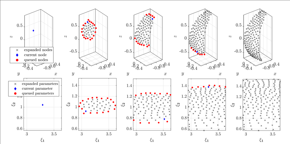
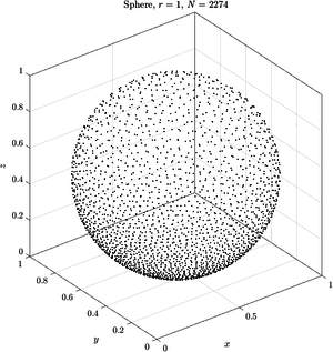
| + | An illustration of the algorithm's progress on a part of a unit sphere can be seen in <xr id="fig:gsf_generation"/> <ref name="GeneralSurfaceFill">U. Duh, G. Kosec and J. Slak, Fast variable density node generation on parametric surfaces with application to mesh-free methods, arXiv preprint arXiv:2005.08767 (2020).</ref>. | ||
| + | |||
| + | <figure id="fig:gsf_generation"> | ||
| + | [[File:gsf_generation.png|1000px|thumb|center|<caption> Progress of the boundary filling algorithm in parametric domain $\Lambda$ (bottom) and main domain $\partial \Omega$ (top). Part of a unit sphere was discretized with $h = 0.08$. </caption>]] | ||
| + | </figure> | ||
| + | |||
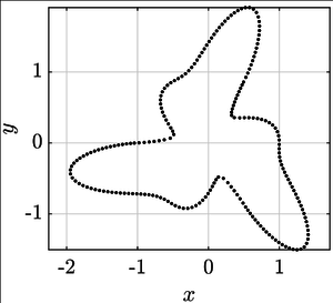
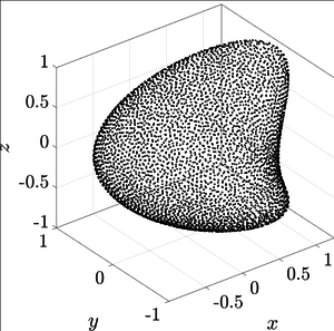
| + | See <xr id="fig:gsf_examples_1"/><ref name="GeneralSurfaceFill"/>, <xr id="fig:gsf_examples_2"/> and <xr id="fig:gsf_examples_3"/><ref name="GeneralSurfaceFill"/>, for examples of discretized curves in 2D and surfaces in 3D. | ||
| + | |||
| + | <figure id="fig:gsf_examples_1"> | ||
| + | [[File:gsf_2d_article.png|thumb|<caption> Example of a 2D domain filled by the boundary filling algorithm. </caption>]] | ||
| + | </figure> | ||
| + | <figure id="fig:gsf_examples_2"> | ||
| + | [[File:3d_simple.png|thumb|<caption> Example of a 3D domain filled by the boundary filling algorithm. </caption>]] | ||
| + | </figure> | ||
| + | <figure id="fig:gsf_examples_3"> | ||
| + | [[File:gsf_3d_article.png|thumb|<caption> Example of a 3D domain filled by the boundary filling algorithm. </caption>]] | ||
| + | </figure> | ||
| + | |||
| + | The boundary filling algorithm can also be used to fill surfaces defined by multiple patches, such as non-uniform rational basis spline (NURBS) models generated by Computer aided design (CAD) software. It is usually beneficial to discretize patch boundaries ($\partial \partial \Omega$) first, since it ensures no gaps of size between $h(\boldsymbol{p})$ and $2h(\boldsymbol{p})$ on patch boundaries. | ||
| + | |||
| + | The algorithm is thoroughly analyzed in <ref name="GeneralSurfaceFill"/>. It is implemented in Medusa as [http://e6.ijs.si/medusa/docs/html/classmm_1_1GeneralSurfaceFill.html GeneralSurfaceFill]. See also [[parametric domains]] example and [[NURBS domains]] example. | ||
| + | |||
| + | === Regularity analysis === | ||
| + | |||
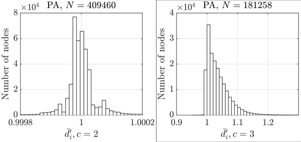
| + | See <xr id="fig:gsf_hist"/><ref name="GeneralSurfaceFill"/> for a distribution of normalized average distances to $c = 2$ nearest neighbors in 2D on a curve from <xr id="fig:gsf_examples_1"/> (left) and $c = 3$ nearest neighbors in 3D on a heart-like surface from <xr id="fig:gsf_examples_3"/> (right) filled with constant $h$. The distribution is satisfactory, since it has a low standard deviation and maximum around $1$. It is even further improved for bigger $N$ (smaller $h$). See also the table below for other global measures of regularity for the same cases as those on the histograms. | ||
| + | |||
| + | <figure id="fig:gsf_hist"> | ||
| + | [[File:gsf_hist.png|thumb|center|600px|<caption> Distribution of normalized distances to $c = 2$ nearest neighbors in 2D (left) and $c = 3$ nearest neighbors in 3D (right) filled with constant $h$. </caption>]] | ||
| + | </figure> | ||
| + | |||
| + | {| class="wikitable" style="margin-left: auto; margin-right: auto; border: none;" | ||
| + | !colspan="6"|Measures of regularity | ||
| + | |- | ||
| + | |dim. | ||
| + | |$\text{mean} \, \bar{d}'_i$ | ||
| + | |$\text{std} \, \bar{d}'_i$ | ||
| + | |$\text{mean} \left(\left(d_i^{\text{max}}\right)' - \left(d_i^{\text{min}}\right)'\right)$ | ||
| + | |$r'_\min$ | ||
| + | |$r'_\max$ | ||
| + | |- | ||
| + | |2D | ||
| + | |$1.0001$ | ||
| + | |$5.1483 \times 10^{-4}$ | ||
| + | |$1.1136 \times 10^{-10}$ | ||
| + | |$0.4622$ | ||
| + | |$0.7808$ | ||
| + | |- | ||
| + | |3D | ||
| + | |$1.0357$ | ||
| + | |$0.0374$ | ||
| + | |$3.8888 \times 10^{-4}$ | ||
| + | |$0.3522$ | ||
| + | |$1.5730$ | ||
| + | |} | ||
| + | |||
| + | === Computational complexity === | ||
| + | |||
| + | Since the boundary filling algorithm is based on the interior filling algorithm, its computational complexity is also equal to<ref name="GeneralSurfaceFill"/> | ||
| + | \begin{equation} | ||
| + | T_{\text{boundary}} = O(P(N) + NnQ(N)+NI(N)), | ||
| + | \end{equation} | ||
| + | where $N$ is the number of generated nodes, $P$ is the precomputation complexity of the spatial search structure, $Q$ is the computational complexity of a radius (nearest neighbor) query and $I$ is the computational complexity of insertions into the spatial search structure. When using a [[K-d tree|''k''-d tree]] spatial search structure this simplifies to | ||
| + | \begin{equation} | ||
| + | T_{\text{boundary, tree}} = O(nN \log N). | ||
| + | \end{equation} | ||
| − | + | Below are some computational times on a laptop computer of filling examples from <xr id="fig:gsf_examples_1"/> and <xr id="fig:gsf_examples_3"/> with $100 \, 000$ nodes, given as a rough reference. | |
| − | == | + | * 2D ($n = 2$): $0.28$ s |
| + | * 3D ($n = 15$): $1.32$ s | ||
| − | + | =References= | |
| + | <references/> | ||
Latest revision as of 19:01, 4 December 2022
Related papers
Contents
Since one of the most attractive features of mesh-free methods is the ability to use nodes without any connectivity information, node placing was considered much easier than mesh generation or simply used existing tools for mesh generation and was thus often disregarded, sometimes implying that any nodes could be used, even if placed at random. It soon turned out that that is not the case, mostly with strong form methods, since many methods require regular nodes for good performance and bad distributions can impact their stability.
One of the key successes of RBF based mesh free methods, such as RBF-generated finite differences
(RBF-FD) is the ability to use highly spatially variable node distributions which can
adapt to irregular geometries and allow for refinement in critical areas.
We present our algorithms below. Their goal is to fill an arbitrary domain $\Omega \subseteq \R^d$ with nodes following the given target spacing function $h(\b{p}): \Omega \to (0, \infty)$, which maps points from $\Omega$ to desired distance to neighboring points.
Please refer to following papers for mode details:
Measures of node regularity
To analyze the regularity of nodes locally, we find $c$ nearest neighbors $\b{p}_{i, j}, j = 1, 2, \dots c$ of each node $\b{p}_i$. Local regularity can now be measured with \begin{align*} \bar{d}_i = \frac{1}{c} \sum_{j =1}^{c}\|\b{p}_i - \b{p}_{i, j}\| & \quad \dots \quad \text{average distance to} \ c \ \text{nearest neighbors}, \\ d_i^{\text{min}} = \min_{j=1, \dots c} \|\b{p}_i - \b{p}_{i, j}\| & \quad \dots \quad \text{minimum distance to} \ c \ \text{nearest neighbors}, \\ d_i^{\text{max}} = \max_{j=1, \dots c} \|\b{p}_i - \b{p}_{i, j}\| & \quad \dots \quad \text{maximum distance to} \ c \ \text{nearest neighbors}. \\ \end{align*} We can also normalize the quantities by scaling them with $h$, thus getting $d'_i = d_i / h(\b{p}_i)$. It is therefore desirable that all the normalised above quantities are approximately equal to $1$.
Global regularity can be assessed by plotting distributions of local regularity measures. For example, a desirable distribution of $\bar{d}'_i$ would have maximum and average approximately equal to $1$ and a low standard deviation. If $h$ is a constant function, a discretization of $\Omega$ with point set $\mathcal{X} = {x_1, \dots, x_N} \subseteq \Omega$ can also be assessed with standard concepts such as[1] \begin{align*} r_{\max, \mathcal{X}} = \sup_{x \in \Omega} \min_{1 \leq j \leq N} \|x - x_j\| & \quad \dots \quad \text{maximum empty sphere radius}, \\ r_{\min, \mathcal{X}} = \frac{1}{2} \min_{i \neq j} \| x_i - x_j \| & \quad \dots \quad \text{separation distance}. \\ \end{align*} Those can also be normalized, getting $r' = r / h$. It is desirable that both $r'_\max$ and $r'_\min$ are approximately equal to $\frac{1}{2}$, however values of $r_\max$ around $2$ (especially when $N$ is small) are also considered good enough. In practice, the maximum empty sphere radius can be numerically estimated by discretizing $\Omega$ with a much smaller nodal spacing $h$ and calculating the maximum empty sphere radius with center in one of the generated nodes.
Filling domain interior
We start with a simple algorithm based on Poisson Disk Sampling (PDS) that results in a relatively tightly packed distribution of nodes. The algorithm beings with a given non-empty set of nodes called "seed nodes". A single seed node placed anywhere in the domain interior is needed to begin the algorithm and if none are provided, one can be chosen at random. However, in the context of PDE discretisations, some nodes on the boundary are usually already known and can be used as seed nodes, possibly along with additional nodes in the interior.
The initial nodes are put in a queue. In each iteration $i$, a new node $\b{p}_i$ is dequeued. Its desired nodal spacing $r_i$ is obtained from the function $h$, $r_i = h(\b{p}_i)$. A set $C_i$ of $n$ new candidates is generated, which lie on the sphere with center $\b{p}_i$ and radius $r_i$. New candidates are spaced uniformly with a random rotation. Candidates that lie outside of the domain or are too close to already existing nodes are rejected. Nearest neighbor search is performed by a spatial search structure, usually a k-d tree is used. Remaining candidates are enqueued and node $\b{p}_i$ is marked as "expanded". The iteration continues until the queue is empty.
An illustration of the algorithm's progress on a unit square can be seen in Figure 1[2].
See Figure 2 and Figure 3 for examples of discretized 2D and 3D domains.
The interior filling algorithm is thoroughly analyzed in [2]. It is implemented in Medusa as GeneralFill.
Regularity analysis
See Figure 4[2] for a distribution of normalized average distances to $c = 3$ nearest neighbors on a 2D unit square (left) and $c = 6$ nearest neighbors on a 3D unit cube (right) filled with constant $h$. The distribution is satisfactory, since it has a lower standard deviation and maximum around $1$. See also the table below for other global measures of regularity for the same cases as those on the histograms.
| Measures of regularity | |||||
|---|---|---|---|---|---|
| dim. | $\text{mean} \, \bar{d}'_i$ | $\text{std} \, \bar{d}'_i$ | $\text{mean} \left(\left(d_i^{\text{max}}\right)' - \left(d_i^{\text{min}}\right)'\right)$ | $r'_\min$ | $r'_\max$ |
| 2D | $1.0416$ | $0.0344$ | $0.0832$ | $0.5000$ | $2.0656$ |
| 3D | $1.0508$ | $0.0418$ | $0.0849$ | $0.5000$ | $2.1023$ |
Computational complexity
Computational complexity of the interior filling algorithm is[2] \begin{equation} T_{\text{interior}} = O(P(N) + NnQ(N)+NI(N)), \end{equation} where $N$ is the number of generated nodes, $P$ is the precomputation complexity of the spatial search structure, $Q$ is the computational complexity of a radius (nearest neighbor) query and $I$ is the computational complexity of insertions into the spatial search structure. When using a k-d tree spatial search structure this simplifies to \begin{equation} T_{\text{interior, tree}} = O(nN \log N). \end{equation} and when using a uniform-grid based spatial search structure[2] (KDGrid in Medusa) it simplifies to \begin{equation} T_{\text{interior, grid}} = O\left(\frac{|\text{obb} \Omega|}{|\Omega|}N + nN\right), \end{equation} where $\text{obb} \Omega$ is the oriented bounding box of $\Omega$.
Below are some computational times on a laptop computer of filling a box with a hole with roughly $100 \, 000$ nodes, given as a rough reference.
- 2D, KDTree: $1.57$ s, of which $5\%$ is candidate generation, $85\%$ is spatial queries and $4\%$ is spatial inserts
- 2D, KDGrid: $0.35$ s, of which $19\%$ is candidate generation, $56\%$ is spatial queries and $0.002\%$ is spatial inserts
- 3D, KDTree: $7.87$ s, of which $6\%$ is candidate generation, $89\%$ is spatial queries and $1\%$ is spatial inserts
- 3D, KDGrid: $2.58$ s, of which $16\%$ is candidate generation, $70\%$ is spatial queries and $0.001\%$ is spatial inserts
Percentages vary slightly with $N$, with larger $N$ increasing spatial query share by $2$ percent points.
Filling parametric surfaces
The algorithm from the previous section can be modified to work on domain boundaries, for example curves in 2D and surfaces in 3D. Let $\partial \Omega$ be a domain boundary parametrized with a regular parametrization $\boldsymbol{r}: \Lambda \subset \mathbb{R}^{d - 1} \to \partial \Omega \subset \mathbb{R}^{d}$ and let $h(\boldsymbol{p})$ be our spacing function.
We can consider our problem as filling the domain $\Lambda$ in a way, that when its nodes are mapped by $\boldsymbol{r}$, they are approximately $h$ apart. The general logic of iteratively expanding nodes can thus stay the same, we only need to generate different candidates. Let $\boldsymbol{\lambda}_i \in \Lambda$ be the parameter we wish to expand. We want to generate candidates $\boldsymbol{\eta}_{i,j} \in H_i \subset \Lambda$ so that \begin{equation} ||\boldsymbol{r}(\boldsymbol{\eta}_{i,j}) - \boldsymbol{r}(\boldsymbol{\lambda}_i)|| = h(\boldsymbol{r}(\boldsymbol{\lambda}_i)). \end{equation} Let \begin{equation} \boldsymbol{\eta}_{i,j} = \boldsymbol{\lambda}_i + \alpha_{i, j} \vec{s}_{i,j}, \end{equation} where $\vec{s}_{i,j}$ is a unit vector and $\alpha_{i, j} > 0$. By using the first order Taylor's expansion we get \begin{align} h(\boldsymbol{r}(\boldsymbol{\lambda}_i)) &\approx ||\boldsymbol{r}(\boldsymbol{\lambda}_i) + \alpha_{i, j} \nabla \boldsymbol{r}(\boldsymbol{\lambda}_i) \vec s_{i, j} - \boldsymbol{r}(\boldsymbol{\lambda}_i)|| = \alpha_{i, j} ||\nabla \boldsymbol{r}(\boldsymbol{\lambda}_i) \vec s_{i, j}||, \\ \alpha_{i, j} &\approx \frac{h(\boldsymbol{r}(\boldsymbol{\lambda}_i))}{||\nabla \boldsymbol{r}(\boldsymbol{\lambda}_i) \vec s_{i, j}||}. \end{align} Therefore, our set of candidates for expansion of $\boldsymbol{\lambda}_i$ can be expressed as \begin{equation} H_i = \left\{ \boldsymbol{\lambda}_i + \frac{h(\boldsymbol{r}(\boldsymbol{\lambda}_i))}{||\nabla \boldsymbol{r}(\boldsymbol{\lambda}_i) \vec s_{i, j}||} \vec{s}_{i, j} ; \vec{s}_{i,j} \in S_i, \right\}. \end{equation} where $S_i$ is a random discretization of a unit sphere and $|S_i| = n$. Now, we can accept candidates that are at least $h(\b{r}(\b{\lambda}_i))$ away from $\b{r}(\b{\lambda}_i)$ and enqueue them for expansion. The boundary filling algorithm terminates when the queue is empty.
An illustration of the algorithm's progress on a part of a unit sphere can be seen in Figure 5 [3].
See Figure 6[3], Figure 7 and Figure 8[3], for examples of discretized curves in 2D and surfaces in 3D.
The boundary filling algorithm can also be used to fill surfaces defined by multiple patches, such as non-uniform rational basis spline (NURBS) models generated by Computer aided design (CAD) software. It is usually beneficial to discretize patch boundaries ($\partial \partial \Omega$) first, since it ensures no gaps of size between $h(\boldsymbol{p})$ and $2h(\boldsymbol{p})$ on patch boundaries.
The algorithm is thoroughly analyzed in [3]. It is implemented in Medusa as GeneralSurfaceFill. See also parametric domains example and NURBS domains example.
Regularity analysis
See Figure 9[3] for a distribution of normalized average distances to $c = 2$ nearest neighbors in 2D on a curve from Figure 6 (left) and $c = 3$ nearest neighbors in 3D on a heart-like surface from Figure 8 (right) filled with constant $h$. The distribution is satisfactory, since it has a low standard deviation and maximum around $1$. It is even further improved for bigger $N$ (smaller $h$). See also the table below for other global measures of regularity for the same cases as those on the histograms.
| Measures of regularity | |||||
|---|---|---|---|---|---|
| dim. | $\text{mean} \, \bar{d}'_i$ | $\text{std} \, \bar{d}'_i$ | $\text{mean} \left(\left(d_i^{\text{max}}\right)' - \left(d_i^{\text{min}}\right)'\right)$ | $r'_\min$ | $r'_\max$ |
| 2D | $1.0001$ | $5.1483 \times 10^{-4}$ | $1.1136 \times 10^{-10}$ | $0.4622$ | $0.7808$ |
| 3D | $1.0357$ | $0.0374$ | $3.8888 \times 10^{-4}$ | $0.3522$ | $1.5730$ |
Computational complexity
Since the boundary filling algorithm is based on the interior filling algorithm, its computational complexity is also equal to[3] \begin{equation} T_{\text{boundary}} = O(P(N) + NnQ(N)+NI(N)), \end{equation} where $N$ is the number of generated nodes, $P$ is the precomputation complexity of the spatial search structure, $Q$ is the computational complexity of a radius (nearest neighbor) query and $I$ is the computational complexity of insertions into the spatial search structure. When using a k-d tree spatial search structure this simplifies to \begin{equation} T_{\text{boundary, tree}} = O(nN \log N). \end{equation}
Below are some computational times on a laptop computer of filling examples from Figure 6 and Figure 8 with $100 \, 000$ nodes, given as a rough reference.
- 2D ($n = 2$): $0.28$ s
- 3D ($n = 15$): $1.32$ s
References
- ↑ H. Wendland, Scattered data approximation, vol. 17, Cambridge university press, 2004.
- ↑ 2.0 2.1 2.2 2.3 2.4 J. Slak and G. Kosec, On generation of node distributions for meshless PDE discretizations, SIAM Journal on Scientific Computing, 41 (2019), pp. A3202–A3229, https://doi.org/10.1137/18M1231456.
- ↑ 3.0 3.1 3.2 3.3 3.4 3.5 U. Duh, G. Kosec and J. Slak, Fast variable density node generation on parametric surfaces with application to mesh-free methods, arXiv preprint arXiv:2005.08767 (2020).

