Difference between revisions of "K-d tree"
m (Grammar) |
|||
| (40 intermediate revisions by 4 users not shown) | |||
| Line 1: | Line 1: | ||
| + | {{DISPLAYTITLE:''k''-d tree}} | ||
In structured meshes, neighborhood relations are implicitly determined by the mapping from the physical to the logical space. | In structured meshes, neighborhood relations are implicitly determined by the mapping from the physical to the logical space. | ||
| − | In unstructured mesh based approaches, support domains can be determined from the mesh | + | In unstructured mesh based approaches, support domains can be determined from the mesh connectivity relations. |
| + | However, in meshless methods, the stencil/support nodes are usually chosen as the nearest $n$ visible nodes. | ||
| + | |||
| + | In order to compute nearest neighbors effectively, fast spatial search structures have been developed, such as [https://en.wikipedia.org/wiki/Octree octree], [https://en.wikipedia.org/wiki/Ball_tree ball tree], [https://en.wikipedia.org/wiki/Cover_tree cover tree] and [https://en.wikipedia.org/wiki/K-d_tree $k$-d tree]. All of these structures first take a list of $N$ points and build a search structure, enabling subsequent queries for $n$ nearest neighbors to be answered in $O(n\log N)$ time. | ||
| + | The $k$-d tree structure is described below to give the reader a basic idea of how such spatial structures store data. | ||
| + | |||
| + | [[File:image_1avj3kcbe157a1ad610k81brmgsj9.png|800px|thumb|<caption> 2D tree example</caption>]] | ||
| + | |||
| + | A $k$-d tree is a binary tree which uses hyperplane space partitioning to divide points into subgroups (subtrees). The plane is chosen based on the depth of the node in a tree. At depth $k$, the $k$-th axis (dimenison) is used to divide the remaining points. Example: in 3 dimensions we have $x$, $y$ and $z$ axes. At root level we decide to divide points according to their $x$ values (we could also do it according to $y$ or $z$ values). Usual criterion for division of points is the median. Thus, at root level, we look for median point by looking at $x$ coordiantes of all points. We put the median point into the root leaf. Remaining points are put into the left and right subtrees. We put the points which have smaller $x$ coorinate into the left subtree and points which have larger $x$ coordinate into the right subtree (or vice versa). We construct the two children nodes of the root from the two subgroups we just created. The procedure is the same, except that we divide the space according to $y$ or $z$ coordinate. We continue this way until we run out of points. The axes used for median search are periodically repeating. | ||
| + | |||
| + | Often, dynamic search structures are needed as well, which support node insertion and removal. In the beginning we were using [http://www.cs.umd.edu/~mount/ANN/ ANN] and [https://www.savarese.com/software/libssrckdtree/ libssrckdtree] | ||
| + | libraries for static and dynamic spatial search structures, respectively. Later, we tested four different publicly available C++ libraries that support at least static spatial search: | ||
| + | |||
| + | * [http://www.cs.umd.edu/~mount/ANN/ ANN] | ||
| + | * [https://www.savarese.com/software/libssrckdtree/ libssrckdtree] | ||
| + | * [http://spatial.sourceforge.net/ spatial] | ||
| + | * [https://github.com/jlblancoc/nanoflann/ nanoflann] | ||
| + | |||
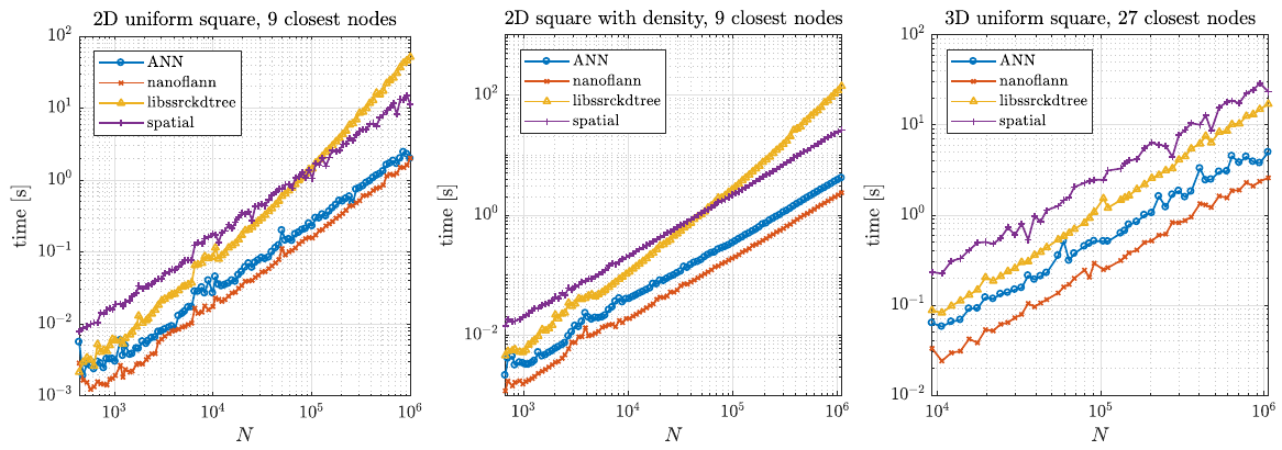
| + | Two typical usage examples for these structures were tested. First, we tested a typical example of finding support domains of $n$ nodes for all nodes, which includes building a tree from a set of points and finding $n$ closest nodes for each point. The results are shown below. | ||
| + | |||
| + | [[File:kdtree_find_support_time.png]] | ||
| + | |||
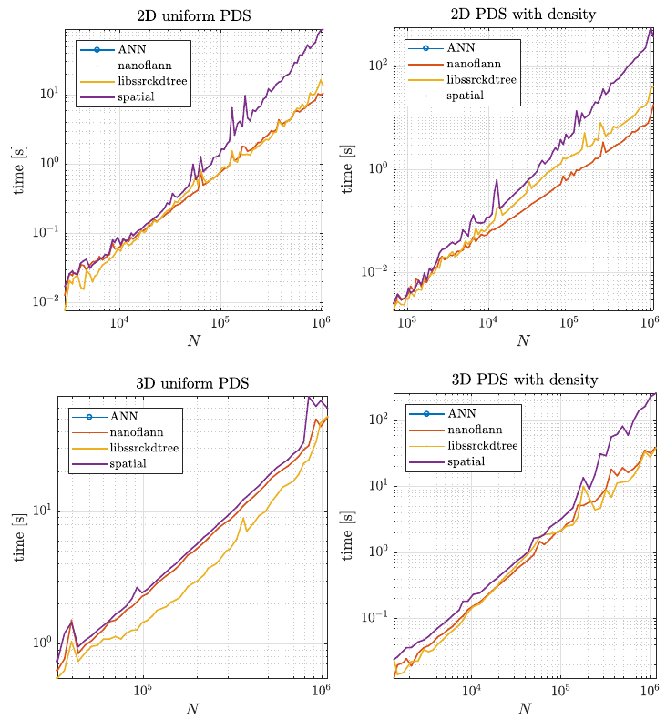
| + | Second, we tested how the structures performed during the node generation process, as described in [[Positioning of computational nodes]] page. Results are shown in figure below. | ||
| + | |||
| + | [[File:kdtree_pds_time.png]] | ||
| + | |||
| + | Besides speed, which was the main factor, we also considered the number of dependencies a library has and how general it is regarding distances and data types. | ||
| + | Overall, we decided to use the [https://github.com/jlblancoc/nanoflann/ nanoflann] library in [http://e6.ijs.si/medusa/ medusa]. Our wrappers are available | ||
| + | as [http://e6.ijs.si/medusa/docs/html/classmm_1_1KDTree.html KDTree] and [http://e6.ijs.si/medusa/docs/html/classmm_1_1KDTreeMutable.html KDTreeMutable]. | ||
| + | |||
| + | The results and reasoning is described more accurately in the technical report [[:File:report.pdf]]. | ||
| − | |||
| − | |||
<!-- | <!-- | ||
| Line 37: | Line 66: | ||
In practical cases, the refinement of the tree stops sooner, when its leaves are represented by list of several nodes, because such a fine grained distribution of leaves as in the presented example is often not beneficial from the computational efficiency point of view. | In practical cases, the refinement of the tree stops sooner, when its leaves are represented by list of several nodes, because such a fine grained distribution of leaves as in the presented example is often not beneficial from the computational efficiency point of view. | ||
--> | --> | ||
| − | |||
== References == | == References == | ||
| − | * Trobec R., Kosec G., | + | * Trobec R., Kosec G., Parallel scientific computing: theory, algorithms, and applications of mesh based and meshless methods: Springer; 2015. |
Latest revision as of 14:30, 16 June 2022
In structured meshes, neighborhood relations are implicitly determined by the mapping from the physical to the logical space. In unstructured mesh based approaches, support domains can be determined from the mesh connectivity relations. However, in meshless methods, the stencil/support nodes are usually chosen as the nearest $n$ visible nodes.
In order to compute nearest neighbors effectively, fast spatial search structures have been developed, such as octree, ball tree, cover tree and $k$-d tree. All of these structures first take a list of $N$ points and build a search structure, enabling subsequent queries for $n$ nearest neighbors to be answered in $O(n\log N)$ time. The $k$-d tree structure is described below to give the reader a basic idea of how such spatial structures store data.
A $k$-d tree is a binary tree which uses hyperplane space partitioning to divide points into subgroups (subtrees). The plane is chosen based on the depth of the node in a tree. At depth $k$, the $k$-th axis (dimenison) is used to divide the remaining points. Example: in 3 dimensions we have $x$, $y$ and $z$ axes. At root level we decide to divide points according to their $x$ values (we could also do it according to $y$ or $z$ values). Usual criterion for division of points is the median. Thus, at root level, we look for median point by looking at $x$ coordiantes of all points. We put the median point into the root leaf. Remaining points are put into the left and right subtrees. We put the points which have smaller $x$ coorinate into the left subtree and points which have larger $x$ coordinate into the right subtree (or vice versa). We construct the two children nodes of the root from the two subgroups we just created. The procedure is the same, except that we divide the space according to $y$ or $z$ coordinate. We continue this way until we run out of points. The axes used for median search are periodically repeating.
Often, dynamic search structures are needed as well, which support node insertion and removal. In the beginning we were using ANN and libssrckdtree libraries for static and dynamic spatial search structures, respectively. Later, we tested four different publicly available C++ libraries that support at least static spatial search:
Two typical usage examples for these structures were tested. First, we tested a typical example of finding support domains of $n$ nodes for all nodes, which includes building a tree from a set of points and finding $n$ closest nodes for each point. The results are shown below.
Second, we tested how the structures performed during the node generation process, as described in Positioning of computational nodes page. Results are shown in figure below.
Besides speed, which was the main factor, we also considered the number of dependencies a library has and how general it is regarding distances and data types. Overall, we decided to use the nanoflann library in medusa. Our wrappers are available as KDTree and KDTreeMutable.
The results and reasoning is described more accurately in the technical report File:report.pdf.
References
- Trobec R., Kosec G., Parallel scientific computing: theory, algorithms, and applications of mesh based and meshless methods: Springer; 2015.


