Difference between revisions of "Natural convection in 3D irregular domain"
| Line 10: | Line 10: | ||
functions, augmented with monomials up to order $2$, with the closest $25$ | functions, augmented with monomials up to order $2$, with the closest $25$ | ||
nodes used as a stencil. For the time discretization time step | nodes used as a stencil. For the time discretization time step | ||
| − | $\Delta t=10^{-3}$ was used for all cases. Domain is discretized with our [[Positioning of computational nodes| | + | $\Delta t=10^{-3}$ was used for all cases. Domain is discretized with our [[Positioning of computational nodes|fill algoritm]] with |
Nodal distance $h=0.025$.. Boundaries with Neumann | Nodal distance $h=0.025$.. Boundaries with Neumann | ||
boundary conditions are additionally treated with ghost nodes [[Ghost nodes (theory)]]. | boundary conditions are additionally treated with ghost nodes [[Ghost nodes (theory)]]. | ||
Revision as of 16:48, 18 May 2019
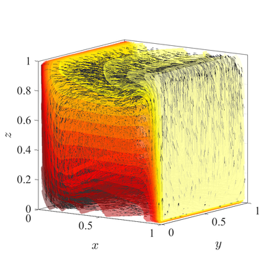
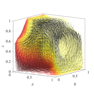
The classical De Vahl Davis natural convection test can be extended to 3D. In below figures steady state temperature contour and velocity quiver plots for Ra$=10^6$ case in 3D are presented. A more quantitative analysis is done by comparing characteristic values, i.e.\ peak positions and values of cross section velocities, with data available in literature~\cite{fusegi1991numerical}. We analyze six different cases, namely Ra$=10^6,10^7,10^8$ in 2D, and Ra$=10^4,10^5,10^6$ in 3D. The comparison in presented in below table.
All spatial operators are discretized using RBF-FD with $r^3$ PHS radial basis functions, augmented with monomials up to order $2$, with the closest $25$ nodes used as a stencil. For the time discretization time step $\Delta t=10^{-3}$ was used for all cases. Domain is discretized with our fill algoritm with Nodal distance $h=0.025$.. Boundaries with Neumann boundary conditions are additionally treated with ghost nodes Ghost nodes (theory).
| Ra | $v_{max}$ | $x$ | $u_{max}$ | $y$ | |||||||||
|---|---|---|---|---|---|---|---|---|---|---|---|---|---|
| present | ref a | ref b | present | ref a | ref b | present | ref a | ref b | present | ref a | ref b | ||
| 2D | $10^6$ | 0.2628 | 0.2604 | 0.2627 | 0.0378 | 0.0380 | 0.0390 | 0.0781 | 0.0765 | 0.0782 | 0.8476 | 0.8510 | 0.0390 |
| $10^7$ | 0.2633 | 0.2580 | 0.2579 | 0.0226 | 0.0230 | 0.0210 | 0.0588 | 0.0547 | 0.0561 | 0.8705 | 0.8880 | 0.0210 | |
| $10^8$ | 0.2557 | 0.2587 | 0.2487 | 0.0149 | 0.0110 | 0.0090 | 0.0314 | 0.0379 | 0.0331 | 0.9189 | 0.9430 | 0.0090 | |
| 3D | $10^4$ | 0.2495 | 0.2218 | 0.2252 | 0.8500 | 0.8873 | 0.8833 | 0.2435 | 0.1968 | 0.2013 | 0.1611 | 0.1799 | 0.1833 |
| $10^5$ | 0.2545 | 0.2442 | 0.2471 | 0.9402 | 0.9317 | 0.9353 | 0.1564 | 0.1426 | 0.1468 | 0.1447 | 0.1493 | 0.1453 | |
| $10^6$ | 0.2564 | 0.2556 | 0.2588 | 0.9614 | 0.9653 | 0.9669 | 0.0841 | 0.0816 | 0.0841 | 0.1435 | 0.1403 | 0.1443 |
[ref a for 2D] @Article{couturier2000performance,
 author    = {Couturier, H. and Sadat, S.},
 title     = {Performance and accuracy of a meshless method for laminar natural convection},
 journal   = {Numerical Heat Transfer: Part B: Fundamentals},
 year      = {2000},
 volume    = {37},
 number    = {4},
 pages     = {455--467},
 doi       = {10.1080/10407790050051146},
 publisher = {Taylor \& Francis},
} [ref b for 2D] @Article{kosec2008solution,
 author    = {Kosec, Gregor and {\v{S}}arler, Bo{\v{z}}idar},
 title     = {Solution of thermo-fluid problems by collocation with local pressure correction},
 journal   = {International Journal of Numerical Methods for Heat \& Fluid Flow},
 year      = {2008},
 volume    = {18},
 number    = {7/8},
 pages     = {868--882},
 doi       = {10.1108/09615530810898999},
 publisher = {Emerald Group Publishing Limited},
} [ref a for 3D] [ref b for 3D]

