Difference between revisions of "Natural convection in 3D irregular domain"
| Line 1: | Line 1: | ||
The classical [[De Vahl Davis natural convection test]] can be extended to 3D. | The classical [[De Vahl Davis natural convection test]] can be extended to 3D. | ||
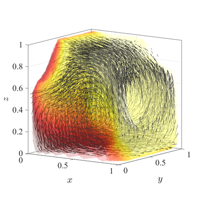
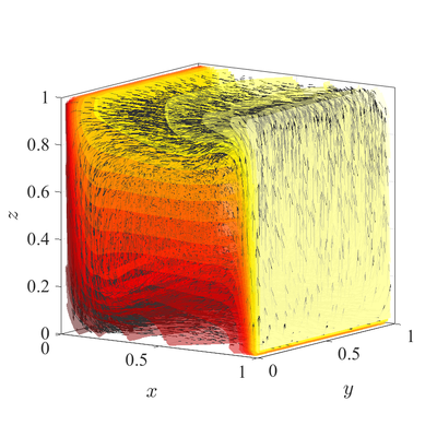
In below figures steady state temperature contour and velocity quiver plots | In below figures steady state temperature contour and velocity quiver plots | ||
| − | for $ | + | for Ra$=10^6$ case in 3D are presented. A more quantitative analysis is done by comparing characteristic values, i.e.\ |
peak positions and values of cross section velocities, with data available in | peak positions and values of cross section velocities, with data available in | ||
literature~\cite{couturier2000performance, kosec2008solution, | literature~\cite{couturier2000performance, kosec2008solution, | ||
Revision as of 16:25, 18 May 2019
The classical De Vahl Davis natural convection test can be extended to 3D. In below figures steady state temperature contour and velocity quiver plots for Ra$=10^6$ case in 3D are presented. A more quantitative analysis is done by comparing characteristic values, i.e.\ peak positions and values of cross section velocities, with data available in literature~\cite{couturier2000performance, kosec2008solution, wang2017numerical, fusegi1991numerical}. We analyze six different cases, namely $\textup{Ra} = 10^6,10^7,10^8$ in 2D, and $\textup{Ra} = 10^4,10^5,10^6$ in 3D. The comparison in presented in~\cref{tab:ff-data}.
All spatial operators are discretized using RBF-FD with $r^3$ PHS radial basis
functions, augmented with monomials up to order $2$, with the closest $25$
nodes used as a stencil. For the time discretization time step
$\Delta t=10^{-3}$ was used for all cases. Nodal distance $h=0.01$ is used for
simulations in 2D and $h=0.25$ for simulations in 3D. Boundaries with Neumann
boundary conditions are additionally treated with ghost nodes Ghost nodes (theory).
\begin{table}[h]
\centering
\caption{Comparison of results computed with RBF-FD on FF nodes and reference
data. }
\label{tab:ff-data}
\renewcommand{\arraystretch}{1.2}
\scalebox{0.68}{
\begin{tabular}{|l|l|l|l|l|l|l|l|l|l|l|l|l|l|}
\cline{2-14}
\multicolumn{1}{c|}{} & \multirow{2}{*}{\textbf{Ra}} &
\multicolumn{3}{c|}{$v_{max}(x, 0.5)'"`UNIQ-MathJax10-QINU`"'x'"`UNIQ-MathJax11-QINU`"'u_{max}(0.5, y)'"`UNIQ-MathJax12-QINU`"'y'"`UNIQ-MathJax13-QINU`"'10^6'"`UNIQ-MathJax14-QINU`"'10^7'"`UNIQ-MathJax15-QINU`"'10^8'"`UNIQ-MathJax16-QINU`"'w_{max}(x, 0.5,0.5)'"`UNIQ-MathJax17-QINU`"'x'"`UNIQ-MathJax18-QINU`"'u_{max}(0.5, 0.5, z)'"`UNIQ-MathJax19-QINU`"'z'"`UNIQ-MathJax20-QINU`"'10^4'"`UNIQ-MathJax21-QINU`"'10^5'"`UNIQ-MathJax22-QINU`"'10^6$ & 0.2564 & 0.2556 & 0.2588 & 0.961 & 0.965 & 0.966 & 0.0841
& 0.0816 & 0.0841 & 0.143 & 0.140 & 0.144
\\ \hline
\end{tabular}
}
\end{table}

