
Downscaling meteorological variables over complex terrain
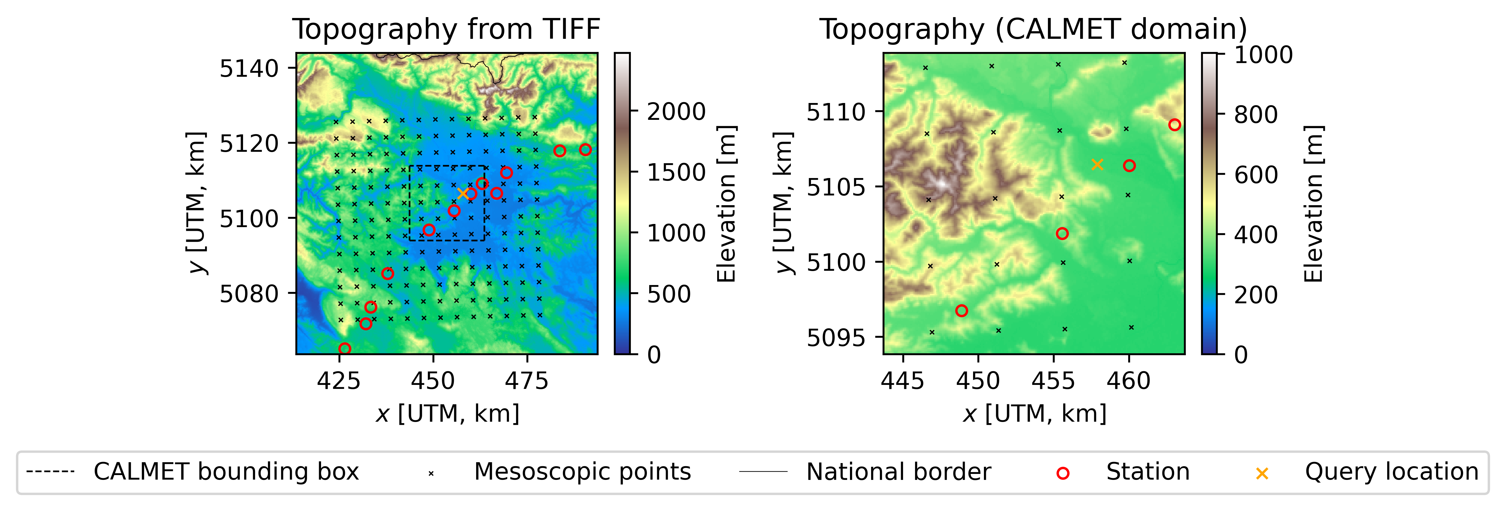
Weather data providers typically provide meteorological variables on a horizontal spatial resolution in order of kilometre or more. Therefore, to capture complex terrain details on smaller scales and to get meteorological variables on specific locations (computational points typically do not correspond to the actual points of interest) downscaling of meteorological fields is required.
Several methods for downscaling mesoscale meteorological data have been proposed, including statistical downscaling, dynamical downscaling and hybrid approaches combining statistical and dynamical methods.
- Statistical downscaling methods use statistical relationships between large-scale atmospheric variables and local weather patterns to produce high-resolution data. Important advances have been just recently made with the rise of machine learning algorithms popularity.
- Dynamic downscaling methods use regional meteorological models that simulate the atmospheric state at a higher resolution than the input data.
- Hybrid approaches combine elements of both statistical and dynamic downscaling.
Unfortunately, to date there is no single best approach, as the performance of downscaling methods varies depending on the desired spatial and temporal resolution of the results and the physical properties of the key variables of interest. Nevertheless, several research groups have reported remarkable agreement between downscaled and observed data.
The goal of this project is to deploy a prototype downscaling model in a framework that is agnostic to the mesoscopic model used for downscaling. In the future, the solution procedure will also be coupled with DiTeR and TrafoFlex where dynamic thermal rating (DTR) models, designed to predict the thermal state of electric power transmission systems, are used to assure the operational safety when subjected to realistic weather conditions and power demands.
P-Lab team


Funding