Cantilever beam

Do you want to go back to Solid Mechanics?

On this page we conduct numerical studies of bending of a cantilever loaded at the end, a common numerical benchmark in elastostatics.

Exact solution

The exact solution to this problem is given by Slaughter (2002) where it is derived for plane stress conditions. Consider a beam of dimensions $L \times D$ having a narrow rectangular cross section. The beam occupies a region of $[0, L] \times [-D/2, D/2]$. The beam is bent by a force $P$ applied at the end $x = 0$ and the other end of the beam is fixed at $x = L$, as illustrated below.

The stresses in such a beam are given as: \begin{equation} \sigma_{xx} = -\frac{Pxy}{I}, \end{equation} \begin{equation} \sigma_{yy} = 0, \end{equation} \begin{equation}\label{eq:sxy} \sigma_{xy} = -\frac{P}{2I}\left(\frac{D^2}{4} - y^2 \right), \end{equation} where $I = D^3/12$ is the moment of inertia.

The exact solution in terms of the displacements in $x$- and $y-$ direction is \begin{align}\label{eq:beam_a1} u_x(x,y) = u(x, y) &= -\frac{Py}{6EI}\left(3(x^2-L^2) -(2+\nu)y^2 + 6 (1+\nu) \frac{D^2}{4}\right) \\ \label{eq:beam_a2} u_y(x,y) = v(x, y) &= \frac{P}{6EI}\left(3\nu x y^2 + x^3 - 3L^2 x + 2L^3\right) \end{align} where $E$ is Young's modulus and $\nu$ is the Poisson ratio. A notebook containing the proof of this equations as well as some plots of the solution is available here: File:cantilever_beam.nb

Copyable C++ code for bending force on the left:

1 std::function<Vec2d(Vec2d)> cantilever_beam_analytical = [=](const Vec2d& p) {
2     double x = p[0], y = p[1];
3     double ux = (P*y*(3*D*D*(1 + v) - 4*(3*L*L - 3*x*x + (2 + v)*y*y)))/(2.*D*D*D*E);
4     double uy = -(P*(3*D*D*(1 + v)*(L - x) + 4*(L-x)*(L-x)*(2*L + x) + 12*v*x*y*y))/(2.*D*D*D*E);
5     return Vec2d(ux, uy);
6 };

Copyable Matlab code for bending force on the left:

 1 function [sxx, syy, sxy, u, v] = cantilever_beam_analytical(x, y, P, L, D, E, nu)
 2 % Evaluates closed form solution to timoshenko cantilever beam.
 3 % P = loading force
 4 % L = length
 5 % D = height
 6 % E = Young's modulus
 7 % nu = Poisson ratio
 8 I = D^3 / 12;
 9 sxx = I.^(-1).*P.*x.*y;
10 syy = zeros(size(x));
11 sxy = (1/2).*I.^(-1).*P.*((1/4).*D.^2+(-1).*y.^2);
12 
13 u = (1/24).*E.^(-1).*I.^(-1).*P.*y.*(3.*D.^2.*(1+nu)-...
14     4.*(3.*L.^2+(-3).*x.^2+(2+nu).*y.^2));
15 v = (-1/24).*E.^(-1).*I.^(-1).*P.*(3.*D.^2.*(1+nu).*(L+(-1).*x)+...
16     4.*(2.*L.^3+(-3).*L.^2.*x+x.^3+3.*nu.*x.*y.^2));
17 end

Numerical solution

For the numerical solution we first choose the following parameters:

• Loading: $P = -1000$ N
• Young's modulus: $E = 3 \times 10^7$ N/m²
• Poisson's ratio: $\nu = 0.3$
• Depth of the beam: $D = 12$ m
• Length of the beam: $L = 48$ m

The unloaded beam is discretized with $40 \times 10$ regular nodes. Since the right end of the beam at $x = L$ is fixed, the displacement boundary conditions are prescribed from the known analytical formulae (\ref{eq:beam_a1}) and (\ref{eq:beam_a2}) : \begin{equation} u_x(L,y) = -\frac{Py}{6EI}\left(-(2+\nu)y^2 + 6 (1+\nu) \frac{D^2}{4}\right); \qquad u_y(L,y) = \frac{P}{2EI}(\nu L y^2) \end{equation} The traction boundary at the left end of the beam ($x=0$) is given by (\ref{eq:sxy}): \begin{equation}\label{eq:trac_a} t_y(L,y) = -\frac{P}{2I}\left(\left(\frac{D}{2}\right)^2 - y^2 \right). \end{equation}

An indicator of the accuracy that can be employed is the strain energy error $e$: \begin{equation} e = \left[ \frac{1}{2} \int_\Omega (\b{\varepsilon}^\mathrm{num} - \b{\varepsilon}^\mathrm{exact})\b{C}(\b{\varepsilon}^\mathrm{num} - \b{\varepsilon}^\mathrm{exact}) d\Omega\right]^{1/2} \end{equation} where $\b{\varepsilon}$ is the strain tensor in vector form, $\b{C}$ the reduced stiffness tensor (a matrix) and $\Omega$ the domain of the calculated solution.

FreeFem++

The required code to solve this problem in FreeFem++ is:

 1  // Parameters
 2  real E = 3.0e7, nu = 0.3;
 3  real P = -1000;
 4  real L = 48, D = 12;
 5  real I = D^3/12;
 6  
 7  // Mesh
 8  mesh Th = square(40,10,[L*x,-D/2+D*y]);
 9  
10  // Macros
11  macro u [ux,uy] // displacement
12  macro v [vx,vy] // test function
13  macro div(u) (dx(u[0])+dy(u[1])) // divergence
14  macro eM(u) [dx(u[0]), dy(u[1]), sqrt(2)*(dx(u[1]) + dy(u[0]))/2] // strain tensor
15  
16  // Finite element space
17  fespace Vh(Th,[P2,P2]);
18  Vh u, v;
19  
20  // Boundary conditions
21  func uxb = -P*y/(6*E*I)*(nu*y^2-2*(1+nu)*y^2+6*D^2/4*(1+nu));
22  func uyb = P/(6*E*I)*(3*nu*L*y^2);
23  func ty = -P/(2*I)*(D^2/4-y^2);
24  
25  // Convert E and nu to plane stress
26  E = E/(1-nu^2); nu = nu/(1-nu);
27  
28  // Lame parameters
29  real mu = E/(2*(1+nu));
30  real lambda = E*nu/((1+nu)*(1-2*nu));
31  
32  // Solve problem
33  solve cantileverBeam(u,v) =
34     int2d(Th)(lambda*div(u)*div(v) + 2*mu*(eM(u)'*eM(v)))
35     - int1d(Th,4)([0,-ty]'*v)
36     + on(2,ux=uxb,uy=uyb);
37  
38  // Plot solution
39  real coef = 1000;
40  Th = movemesh(Th,[x+ux*coef,y+uy*coef]);
41  plot(Th,wait=1);

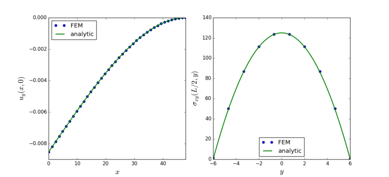
The numerical solutions for beam displacements $u_y(x,0)$ in the axial direction of the beam, and shear stresses $\sigma_{xy}(L/2,y)$ in a cross section at the half lengthwise of the beam, obtained by quadratic finite elements are shown in the figure below. Analytic solutions are shown with continuous lines.

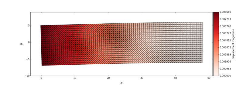
The displaced mesh coloured with the value of the displacement magnitude is presented in the following figure. The displacements are magnified by a factor of 10.

MLSM solution

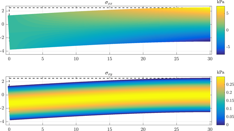
A MLSM solution was compared againts the analytical solution presented above. Resulting stresses are displayed below. All displacements are multiplied by a factor of $10^5$.

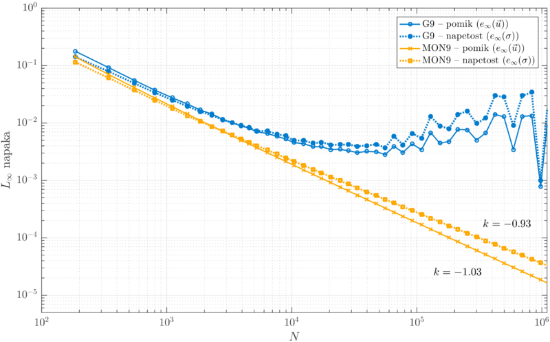
Convergence of stresses and displacements, acquired by solving the implicit system, in $L_\infty$ norm are shown below.

Monomials converge completely regularly with order 2, while Gaussian functions show worse convergence properties.

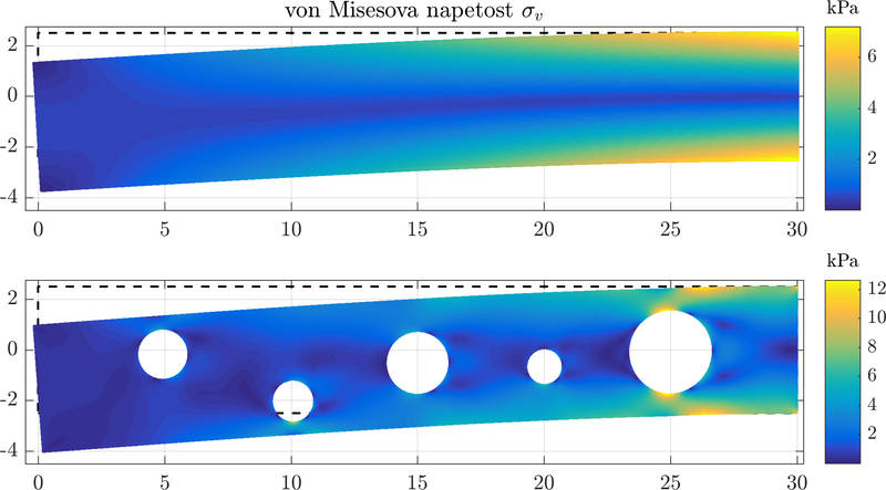
A drilled domain can be analysed to show the generality of the method.

References

- ↑ Augarde, Charles E. and Deeks, Andrew J.. "The use of Timoshenko's exact solution for a cantilever beam in adaptive analysis" , Finite Elements in Analysis and Design. (2008), doi: 10.1016/j.finel.2008.01.010
- ↑ William S. Slaughter (2002). The Linearized Theory of Elasticity, p. 285 - 289. Springer, New York.
- ↑ Liu, Gui-Rong (2003). Mesh free methods: moving beyond the finite element method, p. 161. CRC Press LLC, Boca Raton.